Multiphysics for an SFR Pincell

In this tutorial, you will learn how to:

Couple OpenMC, NekRS, and MOOSE for modeling an SFR pincell
Use MOOSE's reactor module to make meshes for common reactor geometries
Use subcycling to efficiently allocate computational resources

To access this tutorial,


cd cardinal/tutorials/pincell_multiphysics

Geometry and Computational Model

The geometry consists of a single pincell, cooled by sodium. The dimensions and assumed operating conditions are summarized in Table 1. Note that these conditions are not necessarily representative of full-power nuclear reactor conditions, since we elect laminar flow conditions in order to reduce meshing requirements for the sake of a fast-running tutorial. By using laminar flow, we will also use a much lower power density than seen in prototypical systems - but for the sake of a tutorial, all the essential components of multiphysics are present (coupling via power, temperature, and density). In addition, to keep the computational requirements as low as possible for NekRS, the height is only 50 cm (so the eignevalue predicted by OpenMC will also be very low, due to high axial leakage).

Table 1: Geometric and operating specifications for a pincell

Parameter	Value
Fuel pellet diameter, $var element = document.getElementById("moose-equation-8fe8e3da-d157-4d5d-8522-c1ebaab6e10a");katex.render("d_f", element, {displayMode:false,throwOnError:false});$	0.825 cm
Clad outer diameter, $var element = document.getElementById("moose-equation-a1bd007d-c786-410b-8c21-8d16aa75d138");katex.render("d_c", element, {displayMode:false,throwOnError:false});$	0.97 cm
Pin pitch, $var element = document.getElementById("moose-equation-aed620da-bbdb-4364-b5ed-95b57231568b");katex.render("p", element, {displayMode:false,throwOnError:false});$	1.28 cm
Height	50.0 cm
Reynolds number	500.0
Prandtl number	0.00436
Inlet temperature	573 K
Outlet temperature	708 K
Power	250 W

We will couple OpenMC, NekRS, and MOOSE heat conduction in a "single stack" hierarchy, with OpenMC as the main application, MOOSE as the second-level application, and NekRS as the third-level application. This structure is shown in Figure 1, and will allow us to sub-cycle all three codes with respect to one another. Solid black lines indicate data transfers that occur directly from application $var element = document.getElementById("moose-equation-8fc27cb4-d811-43ca-875b-a55d5a3031e5");katex.render("A", element, {displayMode:false,throwOnError:false});$ to application $var element = document.getElementById("moose-equation-a9c877b0-e41a-4c40-84e6-7069e7a48a6c");katex.render("B", element, {displayMode:false,throwOnError:false});$ , while the dashed black lines indicate data transfers that first have to pass through an "intermediate" application.

Figure 1: "Single stack" multiapp hierarchy used in this tutorial.

Like with all Cardinal simulations, Picard iterations are achieved "in time." We have not expounded greatly upon this notion in previous tutorials, so we dedicate some space here. The overall Cardinal simulation has a notion of "time" and a time step index, because all code applications will use a Transient executioner. However, usually only NekRS is solved with non-zero time derivatives. The notion of time-stepping is then used to customize how frequently (i.e., in units of time steps) data is exchanged. To help explain the strategy, represent the time step sizes in NekRS, MOOSE, and OpenMC as $var element = document.getElementById("moose-equation-08b465ed-89e4-4704-8b7e-c14e2dc71975");katex.render("\\Delta t_{nek}", element, {displayMode:false,throwOnError:false});$ , $var element = document.getElementById("moose-equation-a7dd230c-adf5-47c9-982b-e4202339158c");katex.render("\\Delta t_{bison}=M\\Delta t_{nek}", element, {displayMode:false,throwOnError:false});$ , and $var element = document.getElementById("moose-equation-f964ddb1-912a-4f25-be15-cd55ba26c2ee");katex.render("\\Delta t_{openmc}=NM\\Delta t_{nek}", element, {displayMode:false,throwOnError:false});$ , respectively. Selecting $var element = document.getElementById("moose-equation-7a88b7f8-dc71-4dd0-9966-d2afce57d4a9");katex.render("N\\neq1", element, {displayMode:false,throwOnError:false});$ and/or $var element = document.getElementById("moose-equation-e3c720d8-4b55-4e32-9553-20f9689e8506");katex.render("M\\neq1", element, {displayMode:false,throwOnError:false});$ is referred to as "sub-cycling." In other words, NekRS runs $var element = document.getElementById("moose-equation-b2ce7f1d-7436-4a12-a8c5-bc902ff37165");katex.render("M", element, {displayMode:false,throwOnError:false});$ times for each MOOSE solve, while MOOSE runs $var element = document.getElementById("moose-equation-c1d420d5-1298-4f0f-b802-8df782f35c99");katex.render("N", element, {displayMode:false,throwOnError:false});$ times for each OpenMC solve, effectively reducing the total number of MOOSE solves by a factor of $var element = document.getElementById("moose-equation-54a9cb65-45d2-40a8-8c76-7f4bf1c58180");katex.render("M", element, {displayMode:false,throwOnError:false});$ and the total number of OpenMC solves by a factor of $var element = document.getElementById("moose-equation-90e38120-5337-465d-a28f-d807e135ea5b");katex.render("NM", element, {displayMode:false,throwOnError:false});$ compared to the naive approach to exchange data based on the smallest time step across the coupled codes. We can then also reduce the total number of data transfers by only transferring data when needed. Each Picard iteration consists of:

Run an OpenMC $var element = document.getElementById("moose-equation-8e8982ea-c445-40f7-a390-1af02b264c4d");katex.render("k", element, {displayMode:false,throwOnError:false});$ -eigenvalue calculation. Transfer the heat source $var element = document.getElementById("moose-equation-5792ef7b-bed0-42db-ab85-c5d694d2160f");katex.render("\\dot{q}_s", element, {displayMode:false,throwOnError:false});$ to MOOSE.
Repeat $var element = document.getElementById("moose-equation-7ac627ea-c28e-4c7c-a6e9-88eff74da613");katex.render("N", element, {displayMode:false,throwOnError:false});$ times:
- Run a steady-state MOOSE calculation. Transfer the heat flux $var element = document.getElementById("moose-equation-21a4eeb4-5166-47ca-aa67-273b6c2937ff");katex.render("q^{''}", element, {displayMode:false,throwOnError:false});$ to NekRS.
- Run a transient NekRS calculation for $var element = document.getElementById("moose-equation-c2b8da84-dcbc-4bd5-8b6b-c3424ed8a987");katex.render("M", element, {displayMode:false,throwOnError:false});$ time steps. Transfer the wall temperature $var element = document.getElementById("moose-equation-d2abd81c-2262-4108-b64c-c64a8c8cfa5a");katex.render("T_\\text{wall}", element, {displayMode:false,throwOnError:false});$ to MOOSE.
Transfer the solid temperature $var element = document.getElementById("moose-equation-7c604e55-a8fb-4d4f-ae79-35b5741c758f");katex.render("T_s", element, {displayMode:false,throwOnError:false});$ , the fluid temperature $var element = document.getElementById("moose-equation-5f3374ea-af98-4b5f-88dd-f09bebda4776");katex.render("T_f", element, {displayMode:false,throwOnError:false});$ , and the fluid density $var element = document.getElementById("moose-equation-36f64092-b9e2-4198-8854-29ce5a79b6a3");katex.render("\\rho_f", element, {displayMode:false,throwOnError:false});$ to OpenMC.

Figure 2 shows the procedure for an example selection of $var element = document.getElementById("moose-equation-a5107a62-16e5-4e95-b28d-97f48b0fa1c7");katex.render("N=3", element, {displayMode:false,throwOnError:false});$ , meaning that the MOOSE-NekRS sub-solve occurs three times for every OpenMC solve.

Figure 2: Coupling procedure with subcycling for a calculation with OpenMC, MOOSE, and NekRS

In this tutorial, we will use different "time steps" for OpenMC, MOOSE, and NekRS, and we invite you at the end of the tutorial to explore the impact on changing these time step magnitudes to see how you can control the frequency of data transfers.

OpenMC Model

OpenMC is used to solve for the neutron transport and power distribution. The OpenMC model is created using OpenMC's Python API. We will build this geometry using Constructive Solid Geometry (CSG) and divided the pincell into a number of axial layers. On each layer, we will apply temperature and density feedback from the coupled MOOSE-NekRS simulation.

First, we create a number of materials to represent the fuel pellet and cladding. Because these materials will only receive temperature updates (i.e. we will not change their density, because doing so would require us to move cell boundaries in order to preserve mass), we can simply create one material that we will use on all axial layers. Similar to temperature, a unique value of density can also be specified for each cell instance, and so we create a single sodium material for all of the coolant cells that will receive density and temperature feedback from NekRS.

Next, we divide the geometry into a number of axial layers, where on each layer we set up cells to represent the pellet, cladding, and sodium. Each layer is then described by lying between two $var element = document.getElementById("moose-equation-516aa579-3d6f-4114-b3ea-98d6ff4b8cb9");katex.render("z", element, {displayMode:false,throwOnError:false});$ -planes. The boundary condition on the top and bottom faces of the OpenMC model are set to vacuum. Finally, we declare a number of settings related to the initial fission source (uniform over the fissionale regions) and how temperature feedback is applied, and then export all files to XML.

from argparse import ArgumentParser
import numpy as np
import openmc

R = 0.97 / 2.0           # outer radius of the pincell (cm)
Rf = 0.825 / 2.0         # outer radius of the pellet (cm)
pitch = 1.28             # pitch between pincells (cm)
height = 50.0            # height of the pincell (cm)
T_inlet = 573.0          # inlet sodium temperature (K)

ap = ArgumentParser()
ap.add_argument('-n', dest='n_axial', type=int, default=25,
                help='Number of axial cell divisions')

args = ap.parse_args()
N = args.n_axial

all_materials = []

# Then, add the materials for UO2 and zircaloy
uo2 = openmc.Material(name = 'UO2')
uo2.set_density('g/cm3', 10.29769)
uo2.add_element('U', 1.0, enrichment = 2.5)
uo2.add_element('O', 2.0)
all_materials.append(uo2)

zircaloy = openmc.Material(material_id=3, name='Zircaloy 4')
zircaloy.set_density('g/cm3', 6.55)
zircaloy.add_element('Sn', 0.014, 'wo')
zircaloy.add_element('Fe', 0.00165, 'wo')
zircaloy.add_element('Cr', 0.001, 'wo')
zircaloy.add_element('Zr', 0.98335, 'wo')
all_materials.append(zircaloy)

sodium = openmc.Material(name = 'sodium')
sodium.set_density('g/cm3', 1.0)
sodium.add_element('Na', 1.0)
all_materials.append(sodium)

materials = openmc.Materials(all_materials)
materials.export_to_xml()

pincell_surface = openmc.ZCylinder(r = R, name = 'Pincell outer radius')
pellet_surface = openmc.ZCylinder(r = Rf, name = 'Pellet outer radius')
rectangular_prism = openmc.model.RectangularPrism(width = pitch, height = pitch, axis = 'z', origin = (0.0, 0.0), boundary_type = 'reflective')

axial_coords = np.linspace(0.0, height, N + 1)
plane_surfaces = [openmc.ZPlane(z0=coord) for coord in axial_coords]
plane_surfaces[0].boundary_type = 'vacuum'
plane_surfaces[-1].boundary_type = 'vacuum'

fuel_cells = []
clad_cells = []
sodium_cells = []

for i in range(N):
  # these are the two planes that bound the current layer on top and bottom
  layer = +plane_surfaces[i] & -plane_surfaces[i + 1]

  fuel_cells.append(openmc.Cell(fill = uo2, region = -pellet_surface & layer, name = 'Fuel{:n}'.format(i)))
  clad_cells.append(openmc.Cell(fill = zircaloy, region = +pellet_surface & -pincell_surface & layer, name = 'Clad{:n}'.format(i)))
  sodium_cells.append(openmc.Cell(fill = sodium, region = +pincell_surface & layer & -rectangular_prism, name = 'sodium{:n}'.format(i)))

root = openmc.Universe(name = 'root')
root.add_cells(fuel_cells)
root.add_cells(clad_cells)
root.add_cells(sodium_cells)

geometry = openmc.Geometry(root)
geometry.export_to_xml()

settings = openmc.Settings()

# Create an initial uniform spatial source distribution over fissionable zones
lower_left = (-pitch, -pitch, 0.0)
upper_right = (pitch, pitch, height)
uniform_dist = openmc.stats.Box(lower_left, upper_right)

settings.source = openmc.IndependentSource(space=uniform_dist, constraints={'fissionable' : True})

settings.batches = 50
settings.inactive = 10
settings.particles = 10000

settings.temperature = {'default': T_inlet,
                        'method': 'interpolation',
                        'multipole': True,
                        'range': (294.0, 3000.0)}

settings.export_to_xml()

You can create these XML files by running


python pincell.py

Heat Conduction Model

The MOOSE heat transfer module is used to solve for energy conservation in the solid. The solid mesh is shown in Figure 3. This mesh is generated using MOOSE's reactor module, which can be used to make sophisticated meshes of typical reactor geometries such as pin lattices, ducts, and reactor vessels. In this example, we use this module to set up just a single pincell.

Figure 3: Solid mesh

This mesh is described in the solid.i file,

[Mesh<<<{"href": "../syntax/Mesh/index.html"}>>>]
  [pin]
    type = PolygonConcentricCircleMeshGenerator<<<{"description": "This PolygonConcentricCircleMeshGenerator object is designed to mesh a polygon geometry with optional rings centered inside.", "href": "../source/meshgenerators/PolygonConcentricCircleMeshGenerator.html"}>>>
    num_sides<<<{"description": "Number of sides of the polygon."}>>> = 8
    num_sectors_per_side<<<{"description": "Number of azimuthal sectors per polygon side (rotating counterclockwise from top right face)."}>>> = '8 8 8 8 8 8 8 8'
    ring_radii<<<{"description": "Radii of major concentric circles (rings)."}>>> = '${fparse 0.75 * Rf} ${fparse 0.85 * Rf} ${fparse 0.95 * Rf} ${Rf} ${R}'
    ring_intervals<<<{"description": "Number of radial mesh intervals within each major concentric circle excluding their boundary layers."}>>> = '1 1 1 1 2'
    ring_block_ids<<<{"description": "Optional customized block ids for each ring geometry block."}>>> = '2 2 2 2 3'
    polygon_size<<<{"description": "Size of the polygon to be generated (given as either apothem or radius depending on polygon_size_style)."}>>> = '${fparse pin_pitch / 2.0}'
    background_block_ids<<<{"description": "Optional customized block id for the background block."}>>> = '1'
    quad_center_elements<<<{"description": "Whether the center elements are quad or triangular."}>>> = true
  []
  [delete_background]
    type = BlockDeletionGenerator<<<{"description": "Mesh generator which removes elements from the specified subdomains", "href": "../source/meshgenerators/BlockDeletionGenerator.html"}>>>
    input<<<{"description": "The mesh we want to modify"}>>> = pin
    block<<<{"description": "The list of blocks to be deleted"}>>> = '1'
  []
  [fluid]
    type = PolygonConcentricCircleMeshGenerator<<<{"description": "This PolygonConcentricCircleMeshGenerator object is designed to mesh a polygon geometry with optional rings centered inside.", "href": "../source/meshgenerators/PolygonConcentricCircleMeshGenerator.html"}>>>
    num_sides<<<{"description": "Number of sides of the polygon."}>>> = 4
    num_sectors_per_side<<<{"description": "Number of azimuthal sectors per polygon side (rotating counterclockwise from top right face)."}>>> = '10 10 10 10'
    ring_radii<<<{"description": "Radii of major concentric circles (rings)."}>>> = '${R}'
    ring_intervals<<<{"description": "Number of radial mesh intervals within each major concentric circle excluding their boundary layers."}>>> = '1'
    ring_block_ids<<<{"description": "Optional customized block ids for each ring geometry block."}>>> = '500'
    polygon_size<<<{"description": "Size of the polygon to be generated (given as either apothem or radius depending on polygon_size_style)."}>>> = '${fparse pin_pitch / 2.0}'
    background_block_ids<<<{"description": "Optional customized block id for the background block."}>>> = '1'
    background_intervals<<<{"description": "Number of radial meshing intervals in background region (area between rings and ducts) excluding the background's boundary layers."}>>> = 3
  []
  [delete_pin]
    type = BlockDeletionGenerator<<<{"description": "Mesh generator which removes elements from the specified subdomains", "href": "../source/meshgenerators/BlockDeletionGenerator.html"}>>>
    input<<<{"description": "The mesh we want to modify"}>>> = fluid
    block<<<{"description": "The list of blocks to be deleted"}>>> = '500'
  []
  [combine]
    type = CombinerGenerator<<<{"description": "Combine multiple meshes (or copies of one mesh) together into one (disjoint) mesh.  Can optionally translate those meshes before combining them.", "href": "../source/meshgenerators/CombinerGenerator.html"}>>>
    inputs<<<{"description": "The input MeshGenerators.  This can either be N generators or 1 generator.  If only 1 is given then 'positions' must also be given."}>>> = 'delete_background delete_pin'
  []
  [extrude]
    type = AdvancedExtruderGenerator<<<{"description": "Extrudes a 1D mesh into 2D, or a 2D mesh into 3D, can have a variable height for each elevation, variable number of layers within each elevation, variable growth factors of axial element sizes within each elevation and remap subdomain_ids, boundary_ids and element extra integers within each elevation as well as interface boundaries between neighboring elevation layers.", "href": "../source/meshgenerators/AdvancedExtruderGenerator.html"}>>>
    input<<<{"description": "The mesh to extrude"}>>> = combine
    heights<<<{"description": "The height of each elevation"}>>> = ${height}
    num_layers<<<{"description": "The number of layers for each elevation - must be num_elevations in length!"}>>> = ${num_layers}
    direction<<<{"description": "A vector that points in the direction to extrude (note, this will be normalized internally - so don't worry about it here)"}>>> = '0 0 1'
  []
  [rotate]
    type = TransformGenerator<<<{"description": "Applies a linear transform to the entire mesh.", "href": "../source/meshgenerators/TransformGenerator.html"}>>>
    input<<<{"description": "The mesh we want to modify"}>>> = extrude
    transform<<<{"description": "The type of transformation to perform (TRANSLATE, TRANSLATE_CENTER_ORIGIN, TRANSLATE_MIN_ORIGIN, ROTATE, SCALE)"}>>> = ROTATE
    vector_value<<<{"description": "The value to use for the transformation. When using TRANSLATE or SCALE, the xyz coordinates are applied in each direction respectively. When using ROTATE, the values are interpreted as the Euler angles phi, theta and psi given in degrees."}>>> = '45.0 0.0 0.0'
  []

  # We want boundary 5 to be the clad surface, because at the time we made this tutorial
  # that is what the reactor module named this boundary (so we drew that boundary in
  # some figures). If you are making a mesh from scratch, you dont need to go through
  # these gynmastics.
  [delete_5]
    type = BoundaryDeletionGenerator<<<{"description": "Mesh generator which removes side sets", "href": "../source/meshgenerators/BoundaryDeletionGenerator.html"}>>>
    input<<<{"description": "The mesh we want to modify"}>>> = rotate
    boundary_names<<<{"description": "The boundaries to be deleted / kept"}>>> = '5'
  []
  [name_5]
    type = RenameBoundaryGenerator<<<{"description": "Changes the boundary IDs and/or boundary names for a given set of boundaries defined by either boundary ID or boundary name. The changes are independent of ordering. The merging of boundaries is supported.", "href": "../source/meshgenerators/RenameBoundaryGenerator.html"}>>>
    input<<<{"description": "The mesh we want to modify"}>>> = delete_5
    old_boundary<<<{"description": "Elements with these boundary ID(s)/name(s) will be given the new boundary information specified in 'new_boundary'"}>>> = '9'
    new_boundary<<<{"description": "The new boundary ID(s)/name(s) to be given by the boundary elements defined in 'old_boundary'."}>>> = '5'
  []
[]

You can generate this mesh by running


cardinal-opt -i solid.i --mesh-only

which will generate the mesh as the solid_in.e file. You will note in Figure 3 that this mesh actually also includes mesh for the fluid region. In Figure 1, we need a mesh region to "receive" the fluid temperature and density from NekRS, because NekRS cannot directly communicate with OpenMC by skipping the second-level app (MOOSE). Therefore, no solve will occur on this fluid mesh, it simply exists to receive the fluid solution from NekRS before being passed "upwards" to OpenMC. By having this dummy "receiving-only" mesh in the solid application, we will require a few extra steps when we set up the MOOSE heat conduction model in Solid Input Files .

NekRS Model

NekRS is used to solve the incompressible Navier-Stokes equations in non-dimensional form. The NekRS input files needed to solve the incompressible Navier-Stokes equations are:

fluid.re2: NekRS mesh (generated by exo2nek starting from MOOSE-generated meshes, to be discussed shortly)
fluid.par: High-level settings for the solver, boundary condition mappings to sidesets, and the equations to solve
fluid.udf: User-defined C++ functions for on-line postprocessing and model setup
fluid.oudf: User-defined OCCA kernels for boundary conditions and source terms

A detailed description of all of the available parameters, settings, and use cases for these input files is available on the NekRS documentation website. Because the purpose of this analysis is to demonstrate Cardinal's capabilities, only the aspects of NekRS required to understand the present case will be covered.

We first create the mesh using MOOSE's reactor module. The syntax used to build a HEX27 fluid mesh is shown below. A major difference from the dummy fluid receiving portion of the solid mesh is that we now set up some boundary layers on the pincell surfaces, by providing ring_radii (and other parameters) as vectors.

[Mesh<<<{"href": "../syntax/Mesh/index.html"}>>>]
  [pin]
    type = PolygonConcentricCircleMeshGenerator<<<{"description": "This PolygonConcentricCircleMeshGenerator object is designed to mesh a polygon geometry with optional rings centered inside.", "href": "../source/meshgenerators/PolygonConcentricCircleMeshGenerator.html"}>>>
    num_sides<<<{"description": "Number of sides of the polygon."}>>> = 4
    polygon_size<<<{"description": "Size of the polygon to be generated (given as either apothem or radius depending on polygon_size_style)."}>>> = '${fparse pin_pitch / 2.0}'
    num_sectors_per_side<<<{"description": "Number of azimuthal sectors per polygon side (rotating counterclockwise from top right face)."}>>> = '6 6 6 6'
    uniform_mesh_on_sides<<<{"description": "Whether the side elements are reorganized to have a uniform size."}>>> = true

    ring_radii<<<{"description": "Radii of major concentric circles (rings)."}>>> = '${fparse pin_diameter / 2.0} ${bl_0} ${bl_1} ${bl_2} ${bl_3} ${bl_4} ${bl_5}'
    ring_intervals<<<{"description": "Number of radial mesh intervals within each major concentric circle excluding their boundary layers."}>>> = '1 1 1 1 1 1 1'
    ring_block_ids<<<{"description": "Optional customized block ids for each ring geometry block."}>>> = '${fparse fluid_id + 1} ${fluid_id} ${fluid_id} ${fluid_id} ${fluid_id} ${fluid_id} ${fluid_id}'

    background_block_ids<<<{"description": "Optional customized block id for the background block."}>>> = '${fparse fluid_id}'
    background_intervals<<<{"description": "Number of radial meshing intervals in background region (area between rings and ducts) excluding the background's boundary layers."}>>> = 6
  []
  [pin_surface]
    type = SideSetsBetweenSubdomainsGenerator<<<{"description": "MeshGenerator that creates a sideset composed of the nodes located between two or more subdomains.", "href": "../source/meshgenerators/SideSetsBetweenSubdomainsGenerator.html"}>>>
    input<<<{"description": "The mesh we want to modify"}>>> = pin
    primary_block<<<{"description": "The primary set of blocks for which to draw a sideset between"}>>> = ${fluid_id}
    paired_block<<<{"description": "The paired set of blocks for which to draw a sideset between"}>>> = '${fparse fluid_id + 1}'
    new_boundary<<<{"description": "The list of boundary names to create on the supplied subdomain"}>>> = '1'
  []
  [delete_solid]
    type = BlockDeletionGenerator<<<{"description": "Mesh generator which removes elements from the specified subdomains", "href": "../source/meshgenerators/BlockDeletionGenerator.html"}>>>
    input<<<{"description": "The mesh we want to modify"}>>> = pin_surface
    block<<<{"description": "The list of blocks to be deleted"}>>> = '${fparse fluid_id + 1}'
  []
  [rotate]
    type = TransformGenerator<<<{"description": "Applies a linear transform to the entire mesh.", "href": "../source/meshgenerators/TransformGenerator.html"}>>>
    input<<<{"description": "The mesh we want to modify"}>>> = delete_solid
    transform<<<{"description": "The type of transformation to perform (TRANSLATE, TRANSLATE_CENTER_ORIGIN, TRANSLATE_MIN_ORIGIN, ROTATE, SCALE)"}>>> = rotate
    vector_value<<<{"description": "The value to use for the transformation. When using TRANSLATE or SCALE, the xyz coordinates are applied in each direction respectively. When using ROTATE, the values are interpreted as the Euler angles phi, theta and psi given in degrees."}>>> = '45.0 0.0 0.0'
  []

  # We will name boundaries in the mesh for sidesets 2 - 7 using other MOOSE objects.
  # The reactor module does its own sideset naming, so we make sure those IDs are
  # free by deleting whatever the reactor module had.
  [delete_extra_surfaces]
    type = BoundaryDeletionGenerator<<<{"description": "Mesh generator which removes side sets", "href": "../source/meshgenerators/BoundaryDeletionGenerator.html"}>>>
    input<<<{"description": "The mesh we want to modify"}>>> = rotate
    boundary_names<<<{"description": "The boundaries to be deleted / kept"}>>> = '2 3 4 5 6 7'
  []
  [extrude]
    type = AdvancedExtruderGenerator<<<{"description": "Extrudes a 1D mesh into 2D, or a 2D mesh into 3D, can have a variable height for each elevation, variable number of layers within each elevation, variable growth factors of axial element sizes within each elevation and remap subdomain_ids, boundary_ids and element extra integers within each elevation as well as interface boundaries between neighboring elevation layers.", "href": "../source/meshgenerators/AdvancedExtruderGenerator.html"}>>>
    input<<<{"description": "The mesh to extrude"}>>> = delete_extra_surfaces
    direction<<<{"description": "A vector that points in the direction to extrude (note, this will be normalized internally - so don't worry about it here)"}>>> = '0 0 1'
    num_layers<<<{"description": "The number of layers for each elevation - must be num_elevations in length!"}>>> = '${num_layers}'
    heights<<<{"description": "The height of each elevation"}>>> = '${height}'
    bottom_boundary<<<{"description": "The boundary name to set on the bottom boundary. If omitted an ID will be generated."}>>> = '2'
    top_boundary<<<{"description": "The boundary name to set on the top boundary. If omitted an ID will be generated."}>>> = '3'
  []
  [lateral_boundaries]
    type = SideSetsFromNormalsGenerator<<<{"description": "Adds a new named sideset to the mesh for all faces matching the specified normal.", "href": "../source/meshgenerators/SideSetsFromNormalsGenerator.html"}>>>
    input<<<{"description": "The mesh we want to modify"}>>> = extrude
    new_boundary<<<{"description": "The list of boundary names to create on the supplied subdomain"}>>> = '4 5 6 7'
    normals<<<{"description": "A list of normals for which to start painting sidesets"}>>> = '1.0  0.0 0.0
              -1.0  0.0 0.0
               0.0  1.0 0.0
               0.0 -1.0 0.0'
    normal_tol<<<{"description": "If normal is supplied then faces are only added if face_normal.normal_hat >= 1 - normal_tol, where normal_hat = normal/|normal|"}>>> = 1e-6
  []

  second_order<<<{"description": "Converts a first order mesh to a second order mesh.  Note: This is NOT needed if you are reading an actual first order mesh."}>>> = true
[]

However, NekRS requires a HEX20 mesh format. Therefore, we use a NekMeshGenerator to convert from HEX27 to HEX20 format, while also moving the higher-order side nodes on the pincell surface to match the curvilinear elements. The syntax used to convert from the HEX27 fluid mesh to a HEX20 fluid mesh, while preserving the pincell surface, is shown below.

pin_diameter = 0.97e-2     # pin outer diameter
pin_pitch = 1.28e-2        # pin pitch

flow_area = ${fparse pin_pitch * pin_pitch - pi * pin_diameter * pin_diameter / 4.0}
wetted_perimeter = ${fparse pi * pin_diameter}
hydraulic_diameter = ${fparse 4.0 * flow_area / wetted_perimeter}

[Mesh<<<{"href": "../syntax/Mesh/index.html"}>>>]
  [file]
    type = FileMeshGenerator<<<{"description": "Read a mesh from a file.", "href": "../source/meshgenerators/FileMeshGenerator.html"}>>>
    file<<<{"description": "The filename to read."}>>> = fluid_in.e
  []
  [to_hex20]
    type = NekMeshGenerator<<<{"description": "Converts MOOSE meshes to element types needed for Nek (Quad8 or Hex20), while optionally preserving curved edges (which were faceted) in the original mesh.", "href": "../source/meshgenerators/NekMeshGenerator.html"}>>>
    input<<<{"description": "The mesh we want to modify"}>>> = file
    boundary<<<{"description": "Boundary(s) to enforce the curved surface"}>>> = '1'
    radius<<<{"description": "Radius(es) of the surfaces"}>>> = ${fparse pin_diameter / 2.0}
    boundaries_to_rebuild<<<{"description": "Boundary(s) to retain from the original mesh in the new mesh; if not specified, all original boundaries are kept."}>>> = '1 2 3 4 5 6 7'
    layers<<<{"description": "Number of layers to sweep for each boundary when forming the curved surfaces; if not specified, all values default to 0"}>>> = '4'
    geometry_type<<<{"description": "Geometry type to use for moving boundary nodes"}>>> = cylinder
  []
  [scale]
    type = TransformGenerator<<<{"description": "Applies a linear transform to the entire mesh.", "href": "../source/meshgenerators/TransformGenerator.html"}>>>
    input<<<{"description": "The mesh we want to modify"}>>> = to_hex20
    transform<<<{"description": "The type of transformation to perform (TRANSLATE, TRANSLATE_CENTER_ORIGIN, TRANSLATE_MIN_ORIGIN, ROTATE, SCALE)"}>>> = scale
    vector_value<<<{"description": "The value to use for the transformation. When using TRANSLATE or SCALE, the xyz coordinates are applied in each direction respectively. When using ROTATE, the values are interpreted as the Euler angles phi, theta and psi given in degrees."}>>> = '${fparse 1.0 / hydraulic_diameter} ${fparse 1.0 / hydraulic_diameter} ${fparse 1.0 / hydraulic_diameter}'
  []
[]

To generate the meshes, we run:


cardinal-opt -i fluid.i --mesh-only
cardinal-opt -i convert.i --mesh-only
mv convert_in.e convert.exo

and then use the exo2nek utility to convert from the exodus file format (convert.exo) into the custom .re2 format required for NekRS. A depiction of the outputs of the two stages of the mesh generator process are shown in Figure 4. Boundary 2 is the inlet, boundary 3 is the outlet, and boundary 1 is the pincell surface. Boundaries 4 through 7 are the lateral faces of the pincell.

Figure 4: Outputs of the mesh generators used for the NekRS flow domain

Next, the .par file contains problem setup information. This input solves for pressure, velocity, and temperature. In the nondimensional formulation, the "viscosity" becomes $var element = document.getElementById("moose-equation-49b8b6b8-84bc-411c-817f-7a6bec864c56");katex.render("1/Re", element, {displayMode:false,throwOnError:false});$ , where $var element = document.getElementById("moose-equation-deaa0e6a-ea7d-4796-ab27-3129febb4105");katex.render("Re", element, {displayMode:false,throwOnError:false});$ is the Reynolds number, while the "thermal conductivity" becomes $var element = document.getElementById("moose-equation-9c113626-3136-4cd6-bb54-a5b095d28426");katex.render("1/Pe", element, {displayMode:false,throwOnError:false});$ , where $var element = document.getElementById("moose-equation-34d1bf2a-88be-4178-8ae8-198ff079c536");katex.render("Pe", element, {displayMode:false,throwOnError:false});$ is the Peclet number. These nondimensional numbers are used to set various diffusion coefficients in the governing equations with syntax like -500.0, which is equivalent in NekRS syntax to $var element = document.getElementById("moose-equation-e71f2568-06fc-45ba-8ac2-5d4accad0609");katex.render("\\frac{1}{500.0}", element, {displayMode:false,throwOnError:false});$ . On the four lateral faces of the pincell, we set symmetry conditions for velocity.

# Model of single SFR pincell, in non-dimensional form
#
# Pr = 0.00439
# Re = 500.0
# Pe = Re * Pr

[OCCA]
  backend = CPU

[GENERAL]
  stopAt = numSteps
  numSteps = 2000
  dt = 2.5e-3
  timeStepper = tombo2
  writeControl = steps
  writeInterval = 200
  polynomialOrder = 5

[VELOCITY]
  viscosity = -500.0
  density = 1.0
  boundaryTypeMap = w, v, O, symx, symx, symy, symy
  residualTol = 1.0e-7

[PRESSURE]
  residualTol = 1.0e-6

[TEMPERATURE]
  conductivity = -2.195
  rhoCp = 1.0
  boundaryTypeMap = f, t, I, I, I, I, I
  residualTol = 1.0e-6

Next, the .udf file is used to set up initial conditions for velocity, pressure, and temperature. We set uniform axial velocity initial conditions, and temperature to a linear variation from 0 at the inlet to 1 at the outlet.

#include "udf.hpp"

#define LENGTH 42.35158086795113

void UDF_LoadKernels(occa::properties & kernelInfo)
{
}

void UDF_Setup(nrs_t *nrs)
{
  auto mesh = nrs->cds->mesh[0];

  // loop over all the GLL points and assign directly to the solution arrays by
  // indexing according to the field offset necessary to hold the data for each
  // solution component
  int n_gll_points = mesh->Np * mesh->Nelements;
  for (int n = 0; n < n_gll_points; ++n)
  {
    nrs->U[n + 0 * nrs->fieldOffset] = 0.0; // x-velocity
    nrs->U[n + 1 * nrs->fieldOffset] = 0.0; // y-velocity
    nrs->U[n + 2 * nrs->fieldOffset] = 1.0; // z-velocity

    nrs->P[n] = 0.0; // pressure

    nrs->cds->S[n + 0 * nrs->cds->fieldOffset[0]] = mesh->z[n] / LENGTH; // temperature
  }
}

In the .oudf file, we define boundary conditions. On the flux boundary, we will be sending a heat flux from MOOSE into NekRS, so we set the flux equal to the scratch space array, bc->usrwrk[bc->idM].

void velocityDirichletConditions(bcData * bc)
{
  bc->u = 0.0; // x-velocity
  bc->v = 0.0; // y-velocity
  bc->w = 1.0; // z-velocity
}

void scalarDirichletConditions(bcData * bc)
{
  bc->s = 0.0;
}

void scalarNeumannConditions(bcData * bc)
{
  // note: when running with Cardinal, Cardinal will allocate the usrwrk
  // array. If running with NekRS standalone (e.g. nrsmpi), you need to
  // replace the usrwrk with some other value or allocate it youself from
  // the udf and populate it with values.
  bc->flux = bc->usrwrk[bc->idM];
}

Multiphysics Coupling

In this section, OpenMC, NekRS, and MOOSE are coupled for multiphysics modeling of an SFR pincell. This section describes all input files.

OpenMC Input Files

The neutron transport is solved using OpenMC. The input file for this portion of the physics is openmc.i. We begin by defining a number of constants and setting up the mesh mirror. For simplicity, we just use the same mesh as used in the solid application, shown in Figure 3.

inlet_T  = 573.0           # inlet temperature
power = 1e3                # total power (W)
Re = 500.0                 # Reynolds number
outlet_P = 1e6

height = 0.5               # total height of the domain
Df = 0.825e-2              # fuel diameter
pin_diameter = 0.97e-2     # pin outer diameter
pin_pitch = 1.28e-2        # pin pitch

mu = 8.8e-5                # fluid dynamic viscosity
rho = 723.6                # fluid density
Cp = 5512.0                # fluid isobaric specific heat capacity

Rf = ${fparse Df / 2.0}

flow_area = ${fparse pin_pitch * pin_pitch - pi * pin_diameter * pin_diameter / 4.0}
wetted_perimeter = ${fparse pi * pin_diameter}
hydraulic_diameter = ${fparse 4.0 * flow_area / wetted_perimeter}

U_ref = ${fparse Re * mu / rho / hydraulic_diameter}
mdot = ${fparse rho * U_ref * flow_area}
dT = ${fparse power / mdot / Cp}

[Mesh<<<{"href": "../syntax/Mesh/index.html"}>>>]
  [solid]
    type = FileMeshGenerator<<<{"description": "Read a mesh from a file.", "href": "../source/meshgenerators/FileMeshGenerator.html"}>>>
    file<<<{"description": "The filename to read."}>>> = solid_in.e
  []
[]

Next, we define a number of auxiliary variables to be used for diagnostic purposes. With the exception of the FluidDensityAux, none of the following variables are necessary for coupling, but they will allow us to visualize how data is mapped from OpenMC to the mesh mirror. The FluidDensityAux auxiliary kernel on the other hand is used to compute the fluid density, given the temperature variable temp (into which we will write the MOOSE and NekRS temperatures, into different regions of space). Note that we will not send fluid density from NekRS to OpenMC, because the NekRS model uses an incompressible Navier-Stokes model. But to a decent approximation, the fluid density can be approximated solely as a function of temperature using the SodiumSaturationFluidProperties (so named because these properties represent sodium properties at saturation temperature).

[AuxVariables<<<{"href": "../syntax/AuxVariables/index.html"}>>>]
# These auxiliary variables are all just for visualizing the solution and
# the mapping - none of these are part of the calculation sequence

  [material_id]
    family<<<{"description": "Specifies the family of FE shape functions to use for this variable"}>>> = MONOMIAL
    order<<<{"description": "Specifies the order of the FE shape function to use for this variable (additional orders not listed are allowed)"}>>> = CONSTANT
  []
  [cell_temperature]
    family<<<{"description": "Specifies the family of FE shape functions to use for this variable"}>>> = MONOMIAL
    order<<<{"description": "Specifies the order of the FE shape function to use for this variable (additional orders not listed are allowed)"}>>> = CONSTANT
  []
  [cell_density]
    family<<<{"description": "Specifies the family of FE shape functions to use for this variable"}>>> = MONOMIAL
    order<<<{"description": "Specifies the order of the FE shape function to use for this variable (additional orders not listed are allowed)"}>>> = CONSTANT
  []
[]

[AuxKernels<<<{"href": "../syntax/AuxKernels/index.html"}>>>]
  [material_id]
    type = CellMaterialIDAux<<<{"description": "OpenMC fluid material ID, mapped to each MOOSE element", "href": "../source/auxkernels/CellMaterialIDAux.html"}>>>
    variable<<<{"description": "The name of the variable that this object applies to"}>>> = material_id
  []
  [cell_temperature]
    type = CellTemperatureAux<<<{"description": "OpenMC cell temperature (K), mapped to each MOOSE element", "href": "../source/auxkernels/CellTemperatureAux.html"}>>>
    variable<<<{"description": "The name of the variable that this object applies to"}>>> = cell_temperature
  []
  [cell_density]
    type = CellDensityAux<<<{"description": "OpenMC fluid density (kg/m$^3$), mapped to each MOOSE element", "href": "../source/auxkernels/CellDensityAux.html"}>>>
    variable<<<{"description": "The name of the variable that this object applies to"}>>> = cell_density
  []
  [density]
    type = FluidDensityAux<<<{"description": "Computes density from pressure and temperature", "href": "../source/auxkernels/FluidDensityAux.html"}>>>
    variable<<<{"description": "The name of the variable that this object applies to"}>>> = density
    p<<<{"description": "Pressure"}>>> = ${outlet_P}
    T<<<{"description": "Temperature"}>>> = nek_temp
    fp<<<{"description": "The name of the user object for fluid properties"}>>> = sodium
    execute_on<<<{"description": "The list of flag(s) indicating when this object should be executed. For a description of each flag, see https://mooseframework.inl.gov/source/interfaces/SetupInterface.html."}>>> = 'INITIAL TIMESTEP_END'
  []
[]

[FluidProperties<<<{"href": "../syntax/FluidProperties/index.html"}>>>]
  [sodium]
    type = SodiumSaturationFluidProperties<<<{"description": "Fluid properties for liquid sodium at saturation conditions", "href": "../source/fluidproperties/SodiumSaturationFluidProperties.html"}>>>
  []
[]

Next, the [Problem] and [Tallies] blocks define all the parameters related to coupling OpenMC to MOOSE. We will send temperature to OpenMC from blocks 2 and 3 (which represent the solid regions) and we will send temperature and density to OpenMC from block 1 (which represents the fluid region). We add a CellTally to tally the heat source in the fuel.

For this problem, the temperature that gets mapped into OpenMC is sourced from two different applications, which we can customize using the temperature_variables and temperature_blocks parameters. Later in the Transfers block, all data transfers from the sub-applications will write into either solid_temp or nek_temp.

Finally, we provide some additional specifications for how to run OpenMC. We set the number of batches and various triggers that will automatically terminate the OpenMC solution when reaching less than 2% maximum relative uncertainty in the fission power taly and 7.5E-4 standard deviation in $var element = document.getElementById("moose-equation-b4c945a8-b91d-425b-a98a-e6ac08fbc073");katex.render("k", element, {displayMode:false,throwOnError:false});$ .

[Problem<<<{"href": "../syntax/Problem/index.html"}>>>]
  type = OpenMCCellAverageProblem

  power = ${power}
  scaling = 100.0
  density_blocks = '1'
  cell_level = 0

  # This automatically creates these variables and will read from the non-default choice of 'temp'
  temperature_variables = 'solid_temp; nek_temp'
  temperature_blocks = '2 3;        1'

  relaxation = robbins_monro

  # Set some parameters for when we terminate the OpenMC solve in each iteration;
  # this will run a minimum of 30 batches, and after that, terminate once reaching
  # the specified std. dev. of k and rel. err. of the fission tally
  inactive_batches = 20
  batches = 30
  k_trigger = std_dev
  k_trigger_threshold = 7.5e-4
  batch_interval = 50
  max_batches = 1000

  [Tallies<<<{"href": "../syntax/Problem/Tallies/index.html"}>>>]
    [heat_source]
      type = CellTally<<<{"description": "A class which implements distributed cell tallies.", "href": "../source/tallies/CellTally.html"}>>>
      block<<<{"description": "Subdomains for which to add tallies in OpenMC. If not provided, tallies will be applied over the entire domain corresponding to the [Mesh] block."}>>> = '2'
      name<<<{"description": "Auxiliary variable name(s) to use for OpenMC tallies. If not specified, defaults to the names of the scores"}>>> = heat_source

      check_equal_mapped_tally_volumes<<<{"description": "Whether to check if the tallied cells map to regions in the mesh of equal volume. This can be helpful to ensure that the volume normalization of OpenMC's tallies doesn't introduce any unintentional distortion just because the mapped volumes are different. You should only set this to true if your OpenMC tally cells are all the same volume!"}>>> = true

      trigger<<<{"description": "Trigger criterion to determine when OpenMC simulation is complete based on tallies. If multiple scores are specified in 'score, this same trigger is applied to all scores."}>>> = rel_err
      trigger_threshold<<<{"description": "Threshold for the tally trigger"}>>> = 2e-2
      output<<<{"description": "UNRELAXED field(s) to output from OpenMC for each tally score. unrelaxed_tally_std_dev will write the standard deviation of each tally into auxiliary variables named *_std_dev. unrelaxed_tally_rel_error will write the relative standard deviation (unrelaxed_tally_std_dev / unrelaxed_tally) of each tally into auxiliary variables named *_rel_error. unrelaxed_tally will write the raw unrelaxed tally into auxiliary variables named *_raw (replace * with 'name')."}>>> = unrelaxed_tally_std_dev
    []
  []
[]

Next, we set up some initial conditions for the various fields used for coupling.

[ICs<<<{"href": "../syntax/Cardinal/ICs/index.html"}>>>]
  [nek_temp]
    type = FunctionIC<<<{"description": "An initial condition that uses a normal function of x, y, z to produce values (and optionally gradients) for a field variable.", "href": "../source/ics/FunctionIC.html"}>>>
    variable<<<{"description": "The variable this initial condition is supposed to provide values for."}>>> = nek_temp
    function<<<{"description": "The initial condition function."}>>> = temp_ic
  []
  [solid_temp]
    type = FunctionIC<<<{"description": "An initial condition that uses a normal function of x, y, z to produce values (and optionally gradients) for a field variable.", "href": "../source/ics/FunctionIC.html"}>>>
    variable<<<{"description": "The variable this initial condition is supposed to provide values for."}>>> = solid_temp
    function<<<{"description": "The initial condition function."}>>> = temp_ic
  []
  [heat_source]
    type = ConstantIC<<<{"description": "Sets a constant field value.", "href": "../source/ics/ConstantIC.html"}>>>
    variable<<<{"description": "The variable this initial condition is supposed to provide values for."}>>> = heat_source
    block<<<{"description": "The list of blocks (ids or names) that this object will be applied"}>>> = '2'
    value<<<{"description": "The value to be set in IC"}>>> = ${fparse power / (pi * Rf * Rf * height)}
  []
[]

[Functions<<<{"href": "../syntax/Functions/index.html"}>>>]
  [temp_ic]
    type = ParsedFunction<<<{"description": "Function created by parsing a string", "href": "../source/functions/MooseParsedFunction.html"}>>>
    expression<<<{"description": "The user defined function."}>>> = '${inlet_T} + z / ${height} * ${dT}'
  []
[]

Next, we create a MOOSE heat conduction sub-application, and set up transfers of data between OpenMC and MOOSE. These transfers will send solid temperature and fluid temperature from MOOSE up to OpenMC, and a power distribution to MOOSE.

[MultiApps<<<{"href": "../syntax/MultiApps/index.html"}>>>]
  [bison]
    type = TransientMultiApp<<<{"description": "MultiApp for performing coupled simulations with the parent and sub-application both progressing in time.", "href": "../source/multiapps/TransientMultiApp.html"}>>>
    input_files<<<{"description": "The input file for each App.  If this parameter only contains one input file it will be used for all of the Apps.  When using 'positions_from_file' it is also admissable to provide one input_file per file."}>>> = 'bison.i'
    execute_on<<<{"description": "The list of flag(s) indicating when this object should be executed. For a description of each flag, see https://mooseframework.inl.gov/source/interfaces/SetupInterface.html."}>>> = timestep_begin
    sub_cycling<<<{"description": "Set to true to allow this MultiApp to take smaller timesteps than the rest of the simulation.  More than one timestep will be performed for each parent application timestep"}>>> = true
  []
[]

[Transfers<<<{"href": "../syntax/Transfers/index.html"}>>>]
  [solid_temp_to_openmc]
    type = MultiAppGeneralFieldShapeEvaluationTransfer<<<{"description": "Transfers field data at the MultiApp position using the finite element shape functions from the origin application.", "href": "../source/transfers/MultiAppGeneralFieldShapeEvaluationTransfer.html"}>>>
    source_variable<<<{"description": "The variable to transfer from."}>>> = T
    variable<<<{"description": "The auxiliary variable to store the transferred values in."}>>> = solid_temp
    from_multi_app<<<{"description": "The name of the MultiApp to receive data from"}>>> = bison
  []
  [source_to_bison]
    type = MultiAppCopyTransfer<<<{"description": "Copies variables (nonlinear and auxiliary) between multiapps that have identical meshes.", "href": "../source/transfers/MultiAppCopyTransfer.html"}>>>
    source_variable<<<{"description": "The variable to transfer from."}>>> = heat_source
    variable<<<{"description": "The auxiliary variable to store the transferred values in."}>>> = power
    to_multi_app<<<{"description": "The name of the MultiApp to transfer the data to"}>>> = bison
    from_blocks<<<{"description": "Subdomain restriction to transfer from (defaults to all the origin app domain)"}>>> = '2'
    to_blocks<<<{"description": "Subdomain restriction to transfer to, (defaults to all the target app domain)"}>>> = '2'
  []
  [temp_from_nek]
    type = MultiAppGeneralFieldShapeEvaluationTransfer<<<{"description": "Transfers field data at the MultiApp position using the finite element shape functions from the origin application.", "href": "../source/transfers/MultiAppGeneralFieldShapeEvaluationTransfer.html"}>>>
    source_variable<<<{"description": "The variable to transfer from."}>>> = nek_temp
    from_multi_app<<<{"description": "The name of the MultiApp to receive data from"}>>> = bison
    variable<<<{"description": "The auxiliary variable to store the transferred values in."}>>> = nek_temp
  []
[]

Finally, we will use a Transient executioner and add a number of postprocessors for diagnostic purposes.

[Outputs<<<{"href": "../syntax/Outputs/index.html"}>>>]
  exodus<<<{"description": "Output the results using the default settings for Exodus output."}>>> = true
  csv<<<{"description": "Output the scalar variable and postprocessors to a *.csv file using the default CSV output."}>>> = true
[]

[Executioner<<<{"href": "../syntax/Executioner/index.html"}>>>]
  type = Transient
  dt = 0.5
  num_steps = 10
[]

[Postprocessors<<<{"href": "../syntax/Postprocessors/index.html"}>>>]
  [max_tally_rel_err]
    type = TallyRelativeError<<<{"description": "Maximum/minimum tally relative error", "href": "../source/postprocessors/TallyRelativeError.html"}>>>
    value_type<<<{"description": "Whether to give the maximum or minimum tally relative error"}>>> = max
  []
  [k]
    type = KEigenvalue<<<{"description": "k eigenvalue computed by OpenMC", "href": "../source/postprocessors/KEigenvalue.html"}>>>
  []
  [k_std_dev]
    type = KEigenvalue<<<{"description": "k eigenvalue computed by OpenMC", "href": "../source/postprocessors/KEigenvalue.html"}>>>
    output<<<{"description": "The value to output. Options are $k_{eff}$ (mean), the standard deviation of $k_{eff}$ (std_dev), or the relative error of $k_{eff}$ (rel_err)."}>>> = 'std_dev'
  []
[]

Solid Input Files

The conservation of solid energy is solved using the MOOSE heat transfer module. The input file for this portion of the physics is bison.i. We begin by defining a number of constants and setting the mesh.

inlet_T  = 573.0           # inlet temperature
power = 250                # total power (W)
Re = 500.0                 # Reynolds number

height = 0.5               # total height of the domain
Df = 0.825e-2              # fuel diameter
pin_diameter = 0.97e-2     # pin outer diameter
pin_pitch = 1.28e-2        # pin pitch

mu = 8.8e-5                # fluid dynamic viscosity
rho = 723.6                # fluid density
Cp = 5512.0                # fluid isobaric specific heat capacity

Rf = ${fparse Df / 2.0}

flow_area = ${fparse pin_pitch * pin_pitch - pi * pin_diameter * pin_diameter / 4.0}
wetted_perimeter = ${fparse pi * pin_diameter}
hydraulic_diameter = ${fparse 4.0 * flow_area / wetted_perimeter}

U_ref = ${fparse Re * mu / rho / hydraulic_diameter}
mdot = ${fparse rho * U_ref * flow_area}
dT = ${fparse power / mdot / Cp}

[Mesh<<<{"href": "../syntax/Mesh/index.html"}>>>]
  [solid]
    type = FileMeshGenerator<<<{"description": "Read a mesh from a file.", "href": "../source/meshgenerators/FileMeshGenerator.html"}>>>
    file<<<{"description": "The filename to read."}>>> = solid_in.e
  []
[]

Because some blocks in the solid mesh aren't actually used in the solid solve (i.e. the fluid block we will use to receive fluid temperature and density from NekRS), we need to explicitly tell MOOSE to not throw errors related to checking for material properties on every mesh block.

[Problem<<<{"href": "../syntax/Problem/index.html"}>>>]
  type = FEProblem
  material_coverage_check = false
[]

Next, we set up a nonlinear variable T to represent solid temperature and create kernels representing heat conduction with a volumetric heating in the pellet region. In the fluid region, we need to use a NullKernel to indicate that no actual solve happens on this block. On the cladding surface, we will impose a Dirichlet boundary condition given the NekRS fluid temperature. Finally, we set up material properties for the solid blocks using HeatConductionMaterial.

[Variables<<<{"href": "../syntax/Variables/index.html"}>>>]
  [T]
    initial_condition<<<{"description": "Specifies a constant initial condition for this variable"}>>> = ${inlet_T}
  []
[]

[Kernels<<<{"href": "../syntax/Kernels/index.html"}>>>]
  [diffusion]
    type = HeatConduction<<<{"description": "Diffusive heat conduction term $-\\nabla\\cdot(k\\nabla T)$ of the thermal energy conservation equation", "href": "../source/kernels/HeatConduction.html"}>>>
    variable<<<{"description": "The name of the variable that this residual object operates on"}>>> = T
    block<<<{"description": "The list of blocks (ids or names) that this object will be applied"}>>> = '2 3'
  []
  [source]
    type = CoupledForce<<<{"description": "Implements a source term proportional to the value of a coupled variable. Weak form: $(\\psi_i, -\\sigma v)$.", "href": "../source/kernels/CoupledForce.html"}>>>
    variable<<<{"description": "The name of the variable that this residual object operates on"}>>> = T
    v<<<{"description": "The coupled variable which provides the force"}>>> = power
    block<<<{"description": "The list of blocks (ids or names) that this object will be applied"}>>> = '2'
  []
  [null]
    type = NullKernel<<<{"description": "Kernel that sets a zero residual.", "href": "../source/kernels/NullKernel.html"}>>>
    variable<<<{"description": "The name of the variable that this residual object operates on"}>>> = T
    block<<<{"description": "The list of blocks (ids or names) that this object will be applied"}>>> = '1'
  []
[]

[BCs<<<{"href": "../syntax/BCs/index.html"}>>>]
  [pin_outer]
    type = MatchedValueBC<<<{"description": "Implements a NodalBC which equates two different Variables' values on a specified boundary.", "href": "../source/bcs/MatchedValueBC.html"}>>>
    variable<<<{"description": "The name of the variable that this residual object operates on"}>>> = T
    v<<<{"description": "The variable whose value we are to match."}>>> = nek_temp
    boundary<<<{"description": "The list of boundary IDs from the mesh where this object applies"}>>> = '5'
  []
[]

[Materials<<<{"href": "../syntax/Materials/index.html"}>>>]
  [uo2]
    type = HeatConductionMaterial<<<{"description": "General-purpose material model for heat conduction", "href": "../source/materials/HeatConductionMaterial.html"}>>>
    thermal_conductivity<<<{"description": "The thermal conductivity value"}>>> = 5.0
    block<<<{"description": "The list of blocks (ids or names) that this object will be applied"}>>> = '2'
  []
  [clad]
    type = HeatConductionMaterial<<<{"description": "General-purpose material model for heat conduction", "href": "../source/materials/HeatConductionMaterial.html"}>>>
    thermal_conductivity<<<{"description": "The thermal conductivity value"}>>> = 20.0
    block<<<{"description": "The list of blocks (ids or names) that this object will be applied"}>>> = '3'
  []
[]

Next, we declare auxiliary variables to be used for:

coupling to NekRS (to receive the NekRS temperature, nek_temp)
computing the pin surface heat flux (to send heat flux flux to NekRS)
power to represent the volumetric heating received from OpenMC

On each MOOSE-NekRS substep, we will run MOOSE first. For the very first time step, this means we should set an initial condition for the NekRS fluid temperature, which we simply set to a linear function of height. Finally, we create a DiffusionFluxAux to compute the heat flux on the pin surface.

[AuxVariables<<<{"href": "../syntax/AuxVariables/index.html"}>>>]
  [nek_temp]
  []
  [flux]
    family<<<{"description": "Specifies the family of FE shape functions to use for this variable"}>>> = MONOMIAL
    order<<<{"description": "Specifies the order of the FE shape function to use for this variable (additional orders not listed are allowed)"}>>> = CONSTANT
  []
  [power]
    family<<<{"description": "Specifies the family of FE shape functions to use for this variable"}>>> = MONOMIAL
    order<<<{"description": "Specifies the order of the FE shape function to use for this variable (additional orders not listed are allowed)"}>>> = CONSTANT
    initial_condition<<<{"description": "Specifies a constant initial condition for this variable"}>>> = ${fparse power / (pi * Rf * Rf * height)}
  []
[]

[Functions<<<{"href": "../syntax/Functions/index.html"}>>>]
  [axial_fluid_temp]
    type = ParsedFunction<<<{"description": "Function created by parsing a string", "href": "../source/functions/MooseParsedFunction.html"}>>>
    expression<<<{"description": "The user defined function."}>>> = '${inlet_T} + z / ${height} * ${dT}'
  []
[]

[ICs<<<{"href": "../syntax/Cardinal/ICs/index.html"}>>>]
  [nek_temp]
    type = FunctionIC<<<{"description": "An initial condition that uses a normal function of x, y, z to produce values (and optionally gradients) for a field variable.", "href": "../source/ics/FunctionIC.html"}>>>
    variable<<<{"description": "The variable this initial condition is supposed to provide values for."}>>> = nek_temp
    function<<<{"description": "The initial condition function."}>>> = axial_fluid_temp
  []
[]

[AuxKernels<<<{"href": "../syntax/AuxKernels/index.html"}>>>]
  [flux]
    type = DiffusionFluxAux<<<{"description": "Compute components of flux vector for diffusion problems $(\\vec{J} = -D \\nabla C)$.", "href": "../source/auxkernels/DiffusionFluxAux.html"}>>>
    diffusion_variable<<<{"description": "The name of the variable"}>>> = T
    component<<<{"description": "The desired component of flux."}>>> = normal
    diffusivity<<<{"description": "The name of the diffusivity material property that will be used in the flux computation."}>>> = thermal_conductivity
    variable<<<{"description": "The name of the variable that this object applies to"}>>> = flux
    boundary<<<{"description": "The list of boundaries (ids or names) from the mesh where this object applies"}>>> = '5'
  []
[]

Next, we create a NekRS sub-application and set up the data transfers between MOOSE and NekRS. There are four transfers - three are related to sending the temperature and heat flux between MOOSE and NekRS, and the fourth is related to a performance optimization in the NekRS wrapping that will only interpolate data to/from NekRS at the synchronization points with the application "driving" NekRS (in this case, MOOSE heat conduction).

[MultiApps<<<{"href": "../syntax/MultiApps/index.html"}>>>]
  [nek]
    type = TransientMultiApp<<<{"description": "MultiApp for performing coupled simulations with the parent and sub-application both progressing in time.", "href": "../source/multiapps/TransientMultiApp.html"}>>>
    input_files<<<{"description": "The input file for each App.  If this parameter only contains one input file it will be used for all of the Apps.  When using 'positions_from_file' it is also admissable to provide one input_file per file."}>>> = 'nek.i'
    execute_on<<<{"description": "The list of flag(s) indicating when this object should be executed. For a description of each flag, see https://mooseframework.inl.gov/source/interfaces/SetupInterface.html."}>>> = timestep_end
    sub_cycling<<<{"description": "Set to true to allow this MultiApp to take smaller timesteps than the rest of the simulation.  More than one timestep will be performed for each parent application timestep"}>>> = true
  []
[]

[Transfers<<<{"href": "../syntax/Transfers/index.html"}>>>]
  [temperature]
    type = MultiAppGeneralFieldNearestLocationTransfer<<<{"description": "Transfers field data at the MultiApp position by finding the value at the nearest neighbor(s) in the origin application.", "href": "../source/transfers/MultiAppGeneralFieldNearestLocationTransfer.html"}>>>
    source_variable<<<{"description": "The variable to transfer from."}>>> = temperature
    from_multi_app<<<{"description": "The name of the MultiApp to receive data from"}>>> = nek
    variable<<<{"description": "The auxiliary variable to store the transferred values in."}>>> = nek_temp
  []
  [flux]
    type = MultiAppGeneralFieldNearestLocationTransfer<<<{"description": "Transfers field data at the MultiApp position by finding the value at the nearest neighbor(s) in the origin application.", "href": "../source/transfers/MultiAppGeneralFieldNearestLocationTransfer.html"}>>>
    source_variable<<<{"description": "The variable to transfer from."}>>> = flux
    to_multi_app<<<{"description": "The name of the MultiApp to transfer the data to"}>>> = nek
    variable<<<{"description": "The auxiliary variable to store the transferred values in."}>>> = flux
    from_boundaries<<<{"description": "The boundary we are transferring from (if not specified, whole domain is used)."}>>> = '5'
  []
  [flux_integral]
    type = MultiAppPostprocessorTransfer<<<{"description": "Transfers postprocessor data between the master application and sub-application(s).", "href": "../source/transfers/MultiAppPostprocessorTransfer.html"}>>>
    to_postprocessor<<<{"description": "The name of the Postprocessor in the MultiApp to transfer the value to.  This should most likely be a Reporter Postprocessor."}>>> = flux_integral
    from_postprocessor<<<{"description": "The name of the Postprocessor in the Master to transfer the value from."}>>> = flux_integral
    to_multi_app<<<{"description": "The name of the MultiApp to transfer the data to"}>>> = nek
  []
  [send]
    type = MultiAppPostprocessorTransfer<<<{"description": "Transfers postprocessor data between the master application and sub-application(s).", "href": "../source/transfers/MultiAppPostprocessorTransfer.html"}>>>
    to_postprocessor<<<{"description": "The name of the Postprocessor in the MultiApp to transfer the value to.  This should most likely be a Reporter Postprocessor."}>>> = transfer_in
    from_postprocessor<<<{"description": "The name of the Postprocessor in the Master to transfer the value from."}>>> = send
    to_multi_app<<<{"description": "The name of the MultiApp to transfer the data to"}>>> = nek
  []
[]

Next, we set up a number of postprocessors, both for normalizing the total power sent from MOOSE to NekRS, as well as a few diagnostic terms.

[Postprocessors<<<{"href": "../syntax/Postprocessors/index.html"}>>>]
  [send]
    type = Receiver<<<{"description": "Reports the value stored in this processor, which is usually filled in by another object. The Receiver does not compute its own value.", "href": "../source/postprocessors/Receiver.html"}>>>
    default<<<{"description": "The default value"}>>> = 1.0
  []
  [flux_integral]
    # evaluate the total heat flux for normalization
    type = SideDiffusiveFluxIntegral<<<{"description": "Computes the integral of the diffusive flux over the specified boundary", "href": "../source/postprocessors/SideDiffusiveFluxIntegral.html"}>>>
    diffusivity<<<{"description": "The name of the diffusivity material property that will be used in the flux computation. This must be provided if the variable is of finite element type"}>>> = thermal_conductivity
    variable<<<{"description": "The name of the variable which this postprocessor integrates"}>>> = T
    boundary<<<{"description": "The list of boundary IDs from the mesh where this object applies"}>>> = '5'
  []
  [power]
    type = ElementIntegralVariablePostprocessor<<<{"description": "Computes a volume integral of the specified variable", "href": "../source/postprocessors/ElementIntegralVariablePostprocessor.html"}>>>
    variable<<<{"description": "The name of the variable that this object operates on"}>>> = power
    block<<<{"description": "The list of blocks (ids or names) that this object will be applied"}>>> = '2'
    execute_on<<<{"description": "The list of flag(s) indicating when this object should be executed. For a description of each flag, see https://mooseframework.inl.gov/source/interfaces/SetupInterface.html."}>>> = 'transfer initial'
  []
  [max_T_solid]
    type = ElementExtremeValue<<<{"description": "Finds either the min or max elemental value of a variable over the domain.", "href": "../source/postprocessors/ElementExtremeValue.html"}>>>
    variable<<<{"description": "The name of the variable that this postprocessor operates on"}>>> = T
    block<<<{"description": "The list of blocks (ids or names) that this object will be applied"}>>> = '2 3'
  []
[]

Finally, we set up the MOOSE heat conduction solver to use a Transient exeuctioner and specify the output format. Important to note here is that a user-provided choice of M will determine how many NekRS time steps are run for each MOOSE time step.

[Executioner<<<{"href": "../syntax/Executioner/index.html"}>>>]
  type = Transient
  dt = ${fparse M * t_nek * dt0}
  num_steps = 100

  nl_abs_tol = 1e-8
  nl_rel_tol = 1e-16
  petsc_options_value = 'hypre boomeramg'
  petsc_options_iname = '-pc_type -pc_hypre_type'
[]

[Outputs<<<{"href": "../syntax/Outputs/index.html"}>>>]
  exodus<<<{"description": "Output the results using the default settings for Exodus output."}>>> = true
  hide<<<{"description": "A list of the variables and postprocessors that should NOT be output to the Exodus file (may include Variables, ScalarVariables, and Postprocessor names)."}>>> = 'power flux_integral send'
[]

Fluid Input Files

The fluid mass, momentum, and energy transport physics are solved using NekRS. The input file for this portion of the physics is nek.i. We begin by defining a number of constants and by setting up the NekRSMesh mesh mirror. Because we are coupling NekRS via boundary heat transfer to MOOSE, but via volumetric temperature and densities to OpenMC, we need to use a combined boundary and volumetric mesh mirror, so both boundary and volume = true are provided. Because this problem is set up in non-dimensional form, we also need to rescale the mesh to match the units expected by our solid and OpenMC input files.

inlet_T  = 573.0           # inlet temperature
power = 250                # total power (W)
Re = 500.0                 # Reynolds number

pin_diameter = 0.97e-2     # pin outer diameter
pin_pitch = 1.28e-2        # pin pitch

mu = 8.8e-5                # fluid dynamic viscosity
rho = 723.6                # fluid density
Cp = 5512.0                # fluid isobaric specific heat capacity

flow_area = ${fparse pin_pitch * pin_pitch - pi * pin_diameter * pin_diameter / 4.0}
wetted_perimeter = ${fparse pi * pin_diameter}
hydraulic_diameter = ${fparse 4.0 * flow_area / wetted_perimeter}

U_ref = ${fparse Re * mu / rho / hydraulic_diameter}
mdot = ${fparse rho * U_ref * flow_area}
dT = ${fparse power / mdot / Cp}

[Mesh<<<{"href": "../syntax/Mesh/index.html"}>>>]
  type = NekRSMesh
  boundary = '1'
  scaling = ${hydraulic_diameter}
  volume = true
[]

The bulk of the NekRS wrapping is specified with NekRSProblem. The NekRS input files are in non-dimensional form, whereas all other coupled applications use dimensional units. The various *_ref and *_0 parameters define the characteristic scales that were used to non-dimensionalize the NekRS input. We add a NekBoundaryFlux to pass heat flux into NekRS, and a NekFieldVariable to read temperature out.

[Problem<<<{"href": "../syntax/Problem/index.html"}>>>]
  type = NekRSProblem
  casename<<<{"description": "Case name for the NekRS input files; this is <case> in <case>.par, <case>.udf, <case>.oudf, and <case>.re2."}>>> = 'fluid'
  n_usrwrk_slots<<<{"description": "Number of slots to allocate in nrs->usrwrk to hold fields either related to coupling (which will be populated by Cardinal), or other custom usages, such as a distance-to-wall calculation"}>>> = 1

  [Dimensionalize<<<{"href": "../syntax/Problem/Dimensionalize/index.html"}>>>]
    L<<<{"description": "Reference length"}>>> = ${hydraulic_diameter}
    T<<<{"description": "Reference temperature"}>>> = ${inlet_T}
    U<<<{"description": "Reference velocity"}>>> = ${U_ref}
    dT<<<{"description": "Reference temperature difference"}>>> = ${dT}
    rho<<<{"description": "Reference density"}>>> = ${rho}
    Cp<<<{"description": "Reference isobaric specific heat"}>>> = ${Cp}
  []

  [FieldTransfers<<<{"href": "../syntax/Problem/FieldTransfers/index.html"}>>>]
    [flux]
      type = NekBoundaryFlux<<<{"description": "Reads/writes boundary flux data between NekRS and MOOSE."}>>>
      direction<<<{"description": "Direction in which to send data"}>>> = to_nek
      usrwrk_slot<<<{"description": "When 'direction = to_nek', the slot(s) in the usrwrk array to write the incoming data; provide one entry for each quantity being passed"}>>> = 0
    []
    [temperature]
      type = NekFieldVariable<<<{"description": "Reads/writes volumetric field data between NekRS and MOOSE."}>>>
      direction<<<{"description": "Direction in which to send data"}>>> = from_nek
    []
  []

  synchronization_interval = parent_app
[]

Then, we simply set up a Transient executioner with the NekTimeStepper. For postprocessing purposes, we also create two postprocessors to evaluate the average outlet temperature and the maximum fluid temperature. Finally, in order to not overly saturate the screen output, we will only write the Exodus output files and print to the console every 10 Nek time steps.

[Executioner<<<{"href": "../syntax/Executioner/index.html"}>>>]
  type = Transient

  [TimeStepper<<<{"href": "../syntax/Executioner/TimeStepper/index.html"}>>>]
    type = NekTimeStepper
  []
[]

[Outputs<<<{"href": "../syntax/Outputs/index.html"}>>>]
  exodus<<<{"description": "Output the results using the default settings for Exodus output."}>>> = true
  interval = 10
[]

Execution

To run the input files,


mpiexec -np 4 cardinal-opt -i openmc.i

This will produce a number of output files,

openmc_out.e, OpenMC simulation results, mapped to a mesh mirror
openmc_out_bison0.e, MOOSE heat conduction simulation results
openmc_out_bison0_nek0.e, NekRS simulation results, mapped to a mesh mirror
fluid0.f*, NekRS output files

Figure 5 shows the temperature (a) imposed in OpenMC (the output of the CellTemperatureAux) auxiliary kernel; (b) the NekRS fluid temperature; and (c) the MOOSE solid temperature.

Figure 5: Temperatures predicted by NekRS and BISON (middle, right), and what is imposed in OpenMC (left). All images are shown on the same color scale.

The OpenMC power distribution is shown in Figure 6. The small variations of sodium density with temperature cause the power distribution to be fairly symmetric in the axial direction.

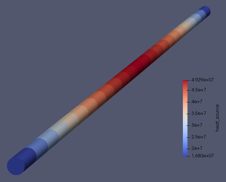
Figure 6: OpenMC predicted power distribution

Finally, Figure 7 shows the fluid and solid temperatures (a) with both phases shown and (b) with just the fluid region highlighted. The very lower power in this demonstration results in fairly small temperature gradients in the fuel, but what is important to note is the coupled solution captures typical conjugate heat transfer temperature distributions in rectangular pincells. You can always extend this tutorial to turbulent conditions and increase the power to display temperature distributions more characteristic of real nuclear systems.

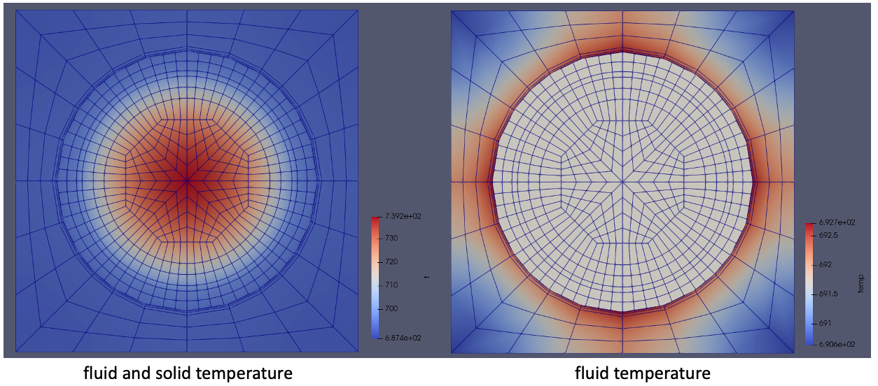
Figure 7: Temperatures predicted by NekRS and BISON on the axial midplane.

In this tutorial, OpenMC, MOOSE, and NekRS each used their own time step. You may want to try re-running this tutorial using different time step sizes in the OpenMC and MOOSE heat conduction input files, to explore how to sub-cycle these codes together.

(tutorials/pincell_multiphysics/pincell.py)

from argparse import ArgumentParser
import numpy as np
import openmc

R = 0.97 / 2.0           # outer radius of the pincell (cm)
Rf = 0.825 / 2.0         # outer radius of the pellet (cm)
pitch = 1.28             # pitch between pincells (cm)
height = 50.0            # height of the pincell (cm)
T_inlet = 573.0          # inlet sodium temperature (K)

ap = ArgumentParser()
ap.add_argument('-n', dest='n_axial', type=int, default=25,
                help='Number of axial cell divisions')

args = ap.parse_args()
N = args.n_axial

all_materials = []

# Then, add the materials for UO2 and zircaloy
uo2 = openmc.Material(name = 'UO2')
uo2.set_density('g/cm3', 10.29769)
uo2.add_element('U', 1.0, enrichment = 2.5)
uo2.add_element('O', 2.0)
all_materials.append(uo2)

zircaloy = openmc.Material(material_id=3, name='Zircaloy 4')
zircaloy.set_density('g/cm3', 6.55)
zircaloy.add_element('Sn', 0.014, 'wo')
zircaloy.add_element('Fe', 0.00165, 'wo')
zircaloy.add_element('Cr', 0.001, 'wo')
zircaloy.add_element('Zr', 0.98335, 'wo')
all_materials.append(zircaloy)

sodium = openmc.Material(name = 'sodium')
sodium.set_density('g/cm3', 1.0)
sodium.add_element('Na', 1.0)
all_materials.append(sodium)

materials = openmc.Materials(all_materials)
materials.export_to_xml()

pincell_surface = openmc.ZCylinder(r = R, name = 'Pincell outer radius')
pellet_surface = openmc.ZCylinder(r = Rf, name = 'Pellet outer radius')
rectangular_prism = openmc.model.RectangularPrism(width = pitch, height = pitch, axis = 'z', origin = (0.0, 0.0), boundary_type = 'reflective')

axial_coords = np.linspace(0.0, height, N + 1)
plane_surfaces = [openmc.ZPlane(z0=coord) for coord in axial_coords]
plane_surfaces[0].boundary_type = 'vacuum'
plane_surfaces[-1].boundary_type = 'vacuum'

fuel_cells = []
clad_cells = []
sodium_cells = []

for i in range(N):
  # these are the two planes that bound the current layer on top and bottom
  layer = +plane_surfaces[i] & -plane_surfaces[i + 1]

  fuel_cells.append(openmc.Cell(fill = uo2, region = -pellet_surface & layer, name = 'Fuel{:n}'.format(i)))
  clad_cells.append(openmc.Cell(fill = zircaloy, region = +pellet_surface & -pincell_surface & layer, name = 'Clad{:n}'.format(i)))
  sodium_cells.append(openmc.Cell(fill = sodium, region = +pincell_surface & layer & -rectangular_prism, name = 'sodium{:n}'.format(i)))

root = openmc.Universe(name = 'root')
root.add_cells(fuel_cells)
root.add_cells(clad_cells)
root.add_cells(sodium_cells)

geometry = openmc.Geometry(root)
geometry.export_to_xml()

settings = openmc.Settings()

# Create an initial uniform spatial source distribution over fissionable zones
lower_left = (-pitch, -pitch, 0.0)
upper_right = (pitch, pitch, height)
uniform_dist = openmc.stats.Box(lower_left, upper_right)

settings.source = openmc.IndependentSource(space=uniform_dist, constraints={'fissionable' : True})

settings.batches = 50
settings.inactive = 10
settings.particles = 10000

settings.temperature = {'default': T_inlet,
                        'method': 'interpolation',
                        'multipole': True,
                        'range': (294.0, 3000.0)}

settings.export_to_xml()

(tutorials/pincell_multiphysics/solid.i)

height = 0.5               # total height of the domain
pin_diameter = 0.97e-2     # pin outer diameter
pin_pitch = 1.28e-2        # pin pitch
Df = 0.825e-2              # fuel diameter
num_layers = 25            # number of layers

Rf = ${fparse Df / 2.0}
R = ${fparse pin_diameter / 2.0}

[Mesh]
  [pin]
    type = PolygonConcentricCircleMeshGenerator
    num_sides = 8
    num_sectors_per_side = '8 8 8 8 8 8 8 8'
    ring_radii = '${fparse 0.75 * Rf} ${fparse 0.85 * Rf} ${fparse 0.95 * Rf} ${Rf} ${R}'
    ring_intervals = '1 1 1 1 2'
    ring_block_ids = '2 2 2 2 3'
    polygon_size = ${fparse pin_pitch / 2.0}
    background_block_ids = '1'
    quad_center_elements = true
  []
  [delete_background]
    type = BlockDeletionGenerator
    input = pin
    block = '1'
  []
  [fluid]
    type = PolygonConcentricCircleMeshGenerator
    num_sides = 4
    num_sectors_per_side = '10 10 10 10'
    ring_radii = '${R}'
    ring_intervals = '1'
    ring_block_ids = '500'
    polygon_size = ${fparse pin_pitch / 2.0}
    background_block_ids = '1'
    background_intervals = 3
  []
  [delete_pin]
    type = BlockDeletionGenerator
    input = fluid
    block = '500'
  []
  [combine]
    type = CombinerGenerator
    inputs = 'delete_background delete_pin'
  []
  [extrude]
    type = AdvancedExtruderGenerator
    input = combine
    heights = ${height}
    num_layers = ${num_layers}
    direction = '0 0 1'
  []
  [rotate]
    type = TransformGenerator
    input = extrude
    transform = ROTATE
    vector_value = '45.0 0.0 0.0'
  []

  # We want boundary 5 to be the clad surface, because at the time we made this tutorial
  # that is what the reactor module named this boundary (so we drew that boundary in
  # some figures). If you are making a mesh from scratch, you dont need to go through
  # these gynmastics.
  [delete_5]
    type = BoundaryDeletionGenerator
    input = rotate
    boundary_names = '5'
  []
  [name_5]
    type = RenameBoundaryGenerator
    input = delete_5
    old_boundary = '9'
    new_boundary = '5'
  []
[]

# The following content is adding postprocessor(s) to check sideset areas.
# The reactor module is unfortunately quite brittle in its assignment of sideset
# IDs, so we want to be extra sure that any changes to sideset numbering are detected
# in our test suite.
[Problem]
  type = FEProblem
  solve = false
[]

[Postprocessors]
  [area_5] # should approximate 0.015236724369910496
    type = AreaPostprocessor
    boundary = '5'
  []
[]

[Executioner]
  type = Steady
[]

[Outputs]
  csv = true
[]

(tutorials/pincell_multiphysics/fluid.i)

height = 0.5               # total height of the domain
pin_diameter = 0.97e-2     # pin outer diameter
pin_pitch = 1.28e-2        # pin pitch
num_layers = 25            # number of layers
fluid_id = 5               # block ID to assign to fluid (only used for bookkeeping)

bl_0 = 0.004855
bl_1 = 0.00486
bl_2 = 0.00488
bl_3 = 0.004934
bl_4 = 0.0050312
bl_5 = 0.0052061600000000005

[Mesh]
  [pin]
    type = PolygonConcentricCircleMeshGenerator
    num_sides = 4
    polygon_size = ${fparse pin_pitch / 2.0}
    num_sectors_per_side = '6 6 6 6'
    uniform_mesh_on_sides = true

    ring_radii = '${fparse pin_diameter / 2.0} ${bl_0} ${bl_1} ${bl_2} ${bl_3} ${bl_4} ${bl_5}'
    ring_intervals = '1 1 1 1 1 1 1'
    ring_block_ids = '${fparse fluid_id + 1} ${fluid_id} ${fluid_id} ${fluid_id} ${fluid_id} ${fluid_id} ${fluid_id}'

    background_block_ids = '${fparse fluid_id}'
    background_intervals = 6
  []
  [pin_surface]
    type = SideSetsBetweenSubdomainsGenerator
    input = pin
    primary_block = ${fluid_id}
    paired_block = ${fparse fluid_id + 1}
    new_boundary = '1'
  []
  [delete_solid]
    type = BlockDeletionGenerator
    input = pin_surface
    block = ${fparse fluid_id + 1}
  []
  [rotate]
    type = TransformGenerator
    input = delete_solid
    transform = rotate
    vector_value = '45.0 0.0 0.0'
  []

  # We will name boundaries in the mesh for sidesets 2 - 7 using other MOOSE objects.
  # The reactor module does its own sideset naming, so we make sure those IDs are
  # free by deleting whatever the reactor module had.
  [delete_extra_surfaces]
    type = BoundaryDeletionGenerator
    input = rotate
    boundary_names = '2 3 4 5 6 7'
  []
  [extrude]
    type = AdvancedExtruderGenerator
    input = delete_extra_surfaces
    direction = '0 0 1'
    num_layers = '${num_layers}'
    heights = '${height}'
    bottom_boundary = '2'
    top_boundary = '3'
  []
  [lateral_boundaries]
    type = SideSetsFromNormalsGenerator
    input = extrude
    new_boundary =  '4 5 6 7'
    normals = '1.0  0.0 0.0
              -1.0  0.0 0.0
               0.0  1.0 0.0
               0.0 -1.0 0.0'
    normal_tol = 1e-6
  []

  second_order = true
[]

# The following content is adding postprocessor(s) to check sideset areas.
# The reactor module is unfortunately quite brittle in its assignment of sideset
# IDs, so we want to be extra sure that any changes to sideset numbering are detected
# in our test suite.
[Problem]
  type = FEProblem
  solve = false
[]

[Postprocessors]
  [area_1] # should approximate 0.015236724369910496
    type = AreaPostprocessor
    boundary = '1'
  []
  [area_2] # should approximate 8.994188680593409e-05
    type = AreaPostprocessor
    boundary = '2'
  []
  [area_3] # should approximate 8.994188680593409e-05
    type = AreaPostprocessor
    boundary = '3'
  []
  [area_4] # should approximate 0.0064
    type = AreaPostprocessor
    boundary = '4'
  []
  [area_5] # should approximate 0.0064
    type = AreaPostprocessor
    boundary = '5'
  []
  [area_6] # should approximate 0.0064
    type = AreaPostprocessor
    boundary = '6'
  []
  [area_7] # should approximate 0.0064
    type = AreaPostprocessor
    boundary = '7'
  []
[]

[Executioner]
  type = Steady
[]

[Outputs]
  csv = true
[]

(tutorials/pincell_multiphysics/convert.i)

pin_diameter = 0.97e-2     # pin outer diameter
pin_pitch = 1.28e-2        # pin pitch

flow_area = ${fparse pin_pitch * pin_pitch - pi * pin_diameter * pin_diameter / 4.0}
wetted_perimeter = ${fparse pi * pin_diameter}
hydraulic_diameter = ${fparse 4.0 * flow_area / wetted_perimeter}

[Mesh]
  [file]
    type = FileMeshGenerator
    file = fluid_in.e
  []
  [to_hex20]
    type = NekMeshGenerator
    input = file
    boundary = '1'
    radius = ${fparse pin_diameter / 2.0}
    boundaries_to_rebuild = '1 2 3 4 5 6 7'
    layers = '4'
    geometry_type = cylinder
  []
  [scale]
    type = TransformGenerator
    input = to_hex20
    transform = scale
    vector_value = '${fparse 1.0 / hydraulic_diameter} ${fparse 1.0 / hydraulic_diameter} ${fparse 1.0 / hydraulic_diameter}'
  []
[]

(tutorials/pincell_multiphysics/fluid.par)

# Model of single SFR pincell, in non-dimensional form
#
# Pr = 0.00439
# Re = 500.0
# Pe = Re * Pr

[OCCA]
  backend = CPU

[GENERAL]
  stopAt = numSteps
  numSteps = 2000
  dt = 2.5e-3
  timeStepper = tombo2
  writeControl = steps
  writeInterval = 200
  polynomialOrder = 5

[VELOCITY]
  viscosity = -500.0
  density = 1.0
  boundaryTypeMap = w, v, O, symx, symx, symy, symy
  residualTol = 1.0e-7

[PRESSURE]
  residualTol = 1.0e-6

[TEMPERATURE]
  conductivity = -2.195
  rhoCp = 1.0
  boundaryTypeMap = f, t, I, I, I, I, I
  residualTol = 1.0e-6

(tutorials/pincell_multiphysics/fluid.udf)

#include "udf.hpp"

#define LENGTH 42.35158086795113

void UDF_LoadKernels(occa::properties & kernelInfo)
{
}

void UDF_Setup(nrs_t *nrs)
{
  auto mesh = nrs->cds->mesh[0];

  // loop over all the GLL points and assign directly to the solution arrays by
  // indexing according to the field offset necessary to hold the data for each
  // solution component
  int n_gll_points = mesh->Np * mesh->Nelements;
  for (int n = 0; n < n_gll_points; ++n)
  {
    nrs->U[n + 0 * nrs->fieldOffset] = 0.0; // x-velocity
    nrs->U[n + 1 * nrs->fieldOffset] = 0.0; // y-velocity
    nrs->U[n + 2 * nrs->fieldOffset] = 1.0; // z-velocity

    nrs->P[n] = 0.0; // pressure

    nrs->cds->S[n + 0 * nrs->cds->fieldOffset[0]] = mesh->z[n] / LENGTH; // temperature
  }
}

(tutorials/pincell_multiphysics/fluid.oudf)

void velocityDirichletConditions(bcData * bc)
{
  bc->u = 0.0; // x-velocity
  bc->v = 0.0; // y-velocity
  bc->w = 1.0; // z-velocity
}

void scalarDirichletConditions(bcData * bc)
{
  bc->s = 0.0;
}

void scalarNeumannConditions(bcData * bc)
{
  // note: when running with Cardinal, Cardinal will allocate the usrwrk
  // array. If running with NekRS standalone (e.g. nrsmpi), you need to
  // replace the usrwrk with some other value or allocate it youself from
  // the udf and populate it with values.
  bc->flux = bc->usrwrk[bc->idM];
}

(tutorials/pincell_multiphysics/openmc.i)

inlet_T  = 573.0           # inlet temperature
power = 1e3                # total power (W)
Re = 500.0                 # Reynolds number
outlet_P = 1e6

height = 0.5               # total height of the domain
Df = 0.825e-2              # fuel diameter
pin_diameter = 0.97e-2     # pin outer diameter
pin_pitch = 1.28e-2        # pin pitch

mu = 8.8e-5                # fluid dynamic viscosity
rho = 723.6                # fluid density
Cp = 5512.0                # fluid isobaric specific heat capacity

Rf = ${fparse Df / 2.0}

flow_area = ${fparse pin_pitch * pin_pitch - pi * pin_diameter * pin_diameter / 4.0}
wetted_perimeter = ${fparse pi * pin_diameter}
hydraulic_diameter = ${fparse 4.0 * flow_area / wetted_perimeter}

U_ref = ${fparse Re * mu / rho / hydraulic_diameter}
mdot = ${fparse rho * U_ref * flow_area}
dT = ${fparse power / mdot / Cp}

[Mesh]
  [solid]
    type = FileMeshGenerator
    file = solid_in.e
  []
[]

[AuxVariables]
# These auxiliary variables are all just for visualizing the solution and
# the mapping - none of these are part of the calculation sequence

  [material_id]
    family = MONOMIAL
    order = CONSTANT
  []
  [cell_temperature]
    family = MONOMIAL
    order = CONSTANT
  []
  [cell_density]
    family = MONOMIAL
    order = CONSTANT
  []
[]

[AuxKernels]
  [material_id]
    type = CellMaterialIDAux
    variable = material_id
  []
  [cell_temperature]
    type = CellTemperatureAux
    variable = cell_temperature
  []
  [cell_density]
    type = CellDensityAux
    variable = cell_density
  []
  [density]
    type = FluidDensityAux
    variable = density
    p = ${outlet_P}
    T = nek_temp
    fp = sodium
    execute_on = 'INITIAL TIMESTEP_END'
  []
[]

[FluidProperties]
  [sodium]
    type = SodiumSaturationFluidProperties
  []
[]

[ICs]
  [nek_temp]
    type = FunctionIC
    variable = nek_temp
    function = temp_ic
  []
  [solid_temp]
    type = FunctionIC
    variable = solid_temp
    function = temp_ic
  []
  [heat_source]
    type = ConstantIC
    variable = heat_source
    block = '2'
    value = ${fparse power / (pi * Rf * Rf * height)}
  []
[]

[Functions]
  [temp_ic]
    type = ParsedFunction
    expression = '${inlet_T} + z / ${height} * ${dT}'
  []
[]

[Problem]
  type = OpenMCCellAverageProblem

  power = ${power}
  scaling = 100.0
  density_blocks = '1'
  cell_level = 0

  # This automatically creates these variables and will read from the non-default choice of 'temp'
  temperature_variables = 'solid_temp; nek_temp'
  temperature_blocks    = '2 3;        1'

  relaxation = robbins_monro

  # Set some parameters for when we terminate the OpenMC solve in each iteration;
  # this will run a minimum of 30 batches, and after that, terminate once reaching
  # the specified std. dev. of k and rel. err. of the fission tally
  inactive_batches = 20
  batches = 30
  k_trigger = std_dev
  k_trigger_threshold = 7.5e-4
  batch_interval = 50
  max_batches = 1000

  [Tallies]
    [heat_source]
      type = CellTally
      block = '2'
      name = heat_source

      check_equal_mapped_tally_volumes = true

      trigger = rel_err
      trigger_threshold = 2e-2
      output = unrelaxed_tally_std_dev
    []
  []
[]

[MultiApps]
  [bison]
    type = TransientMultiApp
    input_files = 'bison.i'
    execute_on = timestep_begin
    sub_cycling = true
  []
[]

[Transfers]
  [solid_temp_to_openmc]
    type = MultiAppGeneralFieldShapeEvaluationTransfer
    source_variable = T
    variable = solid_temp
    from_multi_app = bison
  []
  [source_to_bison]
    type = MultiAppCopyTransfer
    source_variable = heat_source
    variable = power
    to_multi_app = bison
    from_blocks = '2'
    to_blocks = '2'
  []
  [temp_from_nek]
    type = MultiAppGeneralFieldShapeEvaluationTransfer
    source_variable = nek_temp
    from_multi_app = bison
    variable = nek_temp
  []
[]

[Outputs]
  exodus = true
  csv = true
[]

[Executioner]
  type = Transient
  dt = 0.5
  num_steps = 10
[]

[Postprocessors]
  [max_tally_rel_err]
    type = TallyRelativeError
    value_type = max
  []
  [k]
    type = KEigenvalue
  []
  [k_std_dev]
    type = KEigenvalue
    output = 'std_dev'
  []
[]

(tutorials/pincell_multiphysics/openmc.i)

inlet_T  = 573.0           # inlet temperature
power = 1e3                # total power (W)
Re = 500.0                 # Reynolds number
outlet_P = 1e6

height = 0.5               # total height of the domain
Df = 0.825e-2              # fuel diameter
pin_diameter = 0.97e-2     # pin outer diameter
pin_pitch = 1.28e-2        # pin pitch

mu = 8.8e-5                # fluid dynamic viscosity
rho = 723.6                # fluid density
Cp = 5512.0                # fluid isobaric specific heat capacity

Rf = ${fparse Df / 2.0}

flow_area = ${fparse pin_pitch * pin_pitch - pi * pin_diameter * pin_diameter / 4.0}
wetted_perimeter = ${fparse pi * pin_diameter}
hydraulic_diameter = ${fparse 4.0 * flow_area / wetted_perimeter}

U_ref = ${fparse Re * mu / rho / hydraulic_diameter}
mdot = ${fparse rho * U_ref * flow_area}
dT = ${fparse power / mdot / Cp}

[Mesh]
  [solid]
    type = FileMeshGenerator
    file = solid_in.e
  []
[]

[AuxVariables]
# These auxiliary variables are all just for visualizing the solution and
# the mapping - none of these are part of the calculation sequence

  [material_id]
    family = MONOMIAL
    order = CONSTANT
  []
  [cell_temperature]
    family = MONOMIAL
    order = CONSTANT
  []
  [cell_density]
    family = MONOMIAL
    order = CONSTANT
  []
[]

[AuxKernels]
  [material_id]
    type = CellMaterialIDAux
    variable = material_id
  []
  [cell_temperature]
    type = CellTemperatureAux
    variable = cell_temperature
  []
  [cell_density]
    type = CellDensityAux
    variable = cell_density
  []
  [density]
    type = FluidDensityAux
    variable = density
    p = ${outlet_P}
    T = nek_temp
    fp = sodium
    execute_on = 'INITIAL TIMESTEP_END'
  []
[]

[FluidProperties]
  [sodium]
    type = SodiumSaturationFluidProperties
  []
[]

[ICs]
  [nek_temp]
    type = FunctionIC
    variable = nek_temp
    function = temp_ic
  []
  [solid_temp]
    type = FunctionIC
    variable = solid_temp
    function = temp_ic
  []
  [heat_source]
    type = ConstantIC
    variable = heat_source
    block = '2'
    value = ${fparse power / (pi * Rf * Rf * height)}
  []
[]

[Functions]
  [temp_ic]
    type = ParsedFunction
    expression = '${inlet_T} + z / ${height} * ${dT}'
  []
[]

[Problem]
  type = OpenMCCellAverageProblem

  power = ${power}
  scaling = 100.0
  density_blocks = '1'
  cell_level = 0

  # This automatically creates these variables and will read from the non-default choice of 'temp'
  temperature_variables = 'solid_temp; nek_temp'
  temperature_blocks    = '2 3;        1'

  relaxation = robbins_monro

  # Set some parameters for when we terminate the OpenMC solve in each iteration;
  # this will run a minimum of 30 batches, and after that, terminate once reaching
  # the specified std. dev. of k and rel. err. of the fission tally
  inactive_batches = 20
  batches = 30
  k_trigger = std_dev
  k_trigger_threshold = 7.5e-4
  batch_interval = 50
  max_batches = 1000

  [Tallies]
    [heat_source]
      type = CellTally
      block = '2'
      name = heat_source

      check_equal_mapped_tally_volumes = true

      trigger = rel_err
      trigger_threshold = 2e-2
      output = unrelaxed_tally_std_dev
    []
  []
[]

[MultiApps]
  [bison]
    type = TransientMultiApp
    input_files = 'bison.i'
    execute_on = timestep_begin
    sub_cycling = true
  []
[]

[Transfers]
  [solid_temp_to_openmc]
    type = MultiAppGeneralFieldShapeEvaluationTransfer
    source_variable = T
    variable = solid_temp
    from_multi_app = bison
  []
  [source_to_bison]
    type = MultiAppCopyTransfer
    source_variable = heat_source
    variable = power
    to_multi_app = bison
    from_blocks = '2'
    to_blocks = '2'
  []
  [temp_from_nek]
    type = MultiAppGeneralFieldShapeEvaluationTransfer
    source_variable = nek_temp
    from_multi_app = bison
    variable = nek_temp
  []
[]

[Outputs]
  exodus = true
  csv = true
[]

[Executioner]
  type = Transient
  dt = 0.5
  num_steps = 10
[]

[Postprocessors]
  [max_tally_rel_err]
    type = TallyRelativeError
    value_type = max
  []
  [k]
    type = KEigenvalue
  []
  [k_std_dev]
    type = KEigenvalue
    output = 'std_dev'
  []
[]

(tutorials/pincell_multiphysics/openmc.i)

inlet_T  = 573.0           # inlet temperature
power = 1e3                # total power (W)
Re = 500.0                 # Reynolds number
outlet_P = 1e6

height = 0.5               # total height of the domain
Df = 0.825e-2              # fuel diameter
pin_diameter = 0.97e-2     # pin outer diameter
pin_pitch = 1.28e-2        # pin pitch

mu = 8.8e-5                # fluid dynamic viscosity
rho = 723.6                # fluid density
Cp = 5512.0                # fluid isobaric specific heat capacity

Rf = ${fparse Df / 2.0}

flow_area = ${fparse pin_pitch * pin_pitch - pi * pin_diameter * pin_diameter / 4.0}
wetted_perimeter = ${fparse pi * pin_diameter}
hydraulic_diameter = ${fparse 4.0 * flow_area / wetted_perimeter}

U_ref = ${fparse Re * mu / rho / hydraulic_diameter}
mdot = ${fparse rho * U_ref * flow_area}
dT = ${fparse power / mdot / Cp}

[Mesh]
  [solid]
    type = FileMeshGenerator
    file = solid_in.e
  []
[]

[AuxVariables]
# These auxiliary variables are all just for visualizing the solution and
# the mapping - none of these are part of the calculation sequence

  [material_id]
    family = MONOMIAL
    order = CONSTANT
  []
  [cell_temperature]
    family = MONOMIAL
    order = CONSTANT
  []
  [cell_density]
    family = MONOMIAL
    order = CONSTANT
  []
[]

[AuxKernels]
  [material_id]
    type = CellMaterialIDAux
    variable = material_id
  []
  [cell_temperature]
    type = CellTemperatureAux
    variable = cell_temperature
  []
  [cell_density]
    type = CellDensityAux
    variable = cell_density
  []
  [density]
    type = FluidDensityAux
    variable = density
    p = ${outlet_P}
    T = nek_temp
    fp = sodium
    execute_on = 'INITIAL TIMESTEP_END'
  []
[]

[FluidProperties]
  [sodium]
    type = SodiumSaturationFluidProperties
  []
[]

[ICs]
  [nek_temp]
    type = FunctionIC
    variable = nek_temp
    function = temp_ic
  []
  [solid_temp]
    type = FunctionIC
    variable = solid_temp
    function = temp_ic
  []
  [heat_source]
    type = ConstantIC
    variable = heat_source
    block = '2'
    value = ${fparse power / (pi * Rf * Rf * height)}
  []
[]

[Functions]
  [temp_ic]
    type = ParsedFunction
    expression = '${inlet_T} + z / ${height} * ${dT}'
  []
[]

[Problem]
  type = OpenMCCellAverageProblem

  power = ${power}
  scaling = 100.0
  density_blocks = '1'
  cell_level = 0

  # This automatically creates these variables and will read from the non-default choice of 'temp'
  temperature_variables = 'solid_temp; nek_temp'
  temperature_blocks    = '2 3;        1'

  relaxation = robbins_monro

  # Set some parameters for when we terminate the OpenMC solve in each iteration;
  # this will run a minimum of 30 batches, and after that, terminate once reaching
  # the specified std. dev. of k and rel. err. of the fission tally
  inactive_batches = 20
  batches = 30
  k_trigger = std_dev
  k_trigger_threshold = 7.5e-4
  batch_interval = 50
  max_batches = 1000

  [Tallies]
    [heat_source]
      type = CellTally
      block = '2'
      name = heat_source

      check_equal_mapped_tally_volumes = true

      trigger = rel_err
      trigger_threshold = 2e-2
      output = unrelaxed_tally_std_dev
    []
  []
[]

[MultiApps]
  [bison]
    type = TransientMultiApp
    input_files = 'bison.i'
    execute_on = timestep_begin
    sub_cycling = true
  []
[]

[Transfers]
  [solid_temp_to_openmc]
    type = MultiAppGeneralFieldShapeEvaluationTransfer
    source_variable = T
    variable = solid_temp
    from_multi_app = bison
  []
  [source_to_bison]
    type = MultiAppCopyTransfer
    source_variable = heat_source
    variable = power
    to_multi_app = bison
    from_blocks = '2'
    to_blocks = '2'
  []
  [temp_from_nek]
    type = MultiAppGeneralFieldShapeEvaluationTransfer
    source_variable = nek_temp
    from_multi_app = bison
    variable = nek_temp
  []
[]

[Outputs]
  exodus = true
  csv = true
[]

[Executioner]
  type = Transient
  dt = 0.5
  num_steps = 10
[]

[Postprocessors]
  [max_tally_rel_err]
    type = TallyRelativeError
    value_type = max
  []
  [k]
    type = KEigenvalue
  []
  [k_std_dev]
    type = KEigenvalue
    output = 'std_dev'
  []
[]

(tutorials/pincell_multiphysics/openmc.i)

inlet_T  = 573.0           # inlet temperature
power = 1e3                # total power (W)
Re = 500.0                 # Reynolds number
outlet_P = 1e6

height = 0.5               # total height of the domain
Df = 0.825e-2              # fuel diameter
pin_diameter = 0.97e-2     # pin outer diameter
pin_pitch = 1.28e-2        # pin pitch

mu = 8.8e-5                # fluid dynamic viscosity
rho = 723.6                # fluid density
Cp = 5512.0                # fluid isobaric specific heat capacity

Rf = ${fparse Df / 2.0}

flow_area = ${fparse pin_pitch * pin_pitch - pi * pin_diameter * pin_diameter / 4.0}
wetted_perimeter = ${fparse pi * pin_diameter}
hydraulic_diameter = ${fparse 4.0 * flow_area / wetted_perimeter}

U_ref = ${fparse Re * mu / rho / hydraulic_diameter}
mdot = ${fparse rho * U_ref * flow_area}
dT = ${fparse power / mdot / Cp}

[Mesh]
  [solid]
    type = FileMeshGenerator
    file = solid_in.e
  []
[]

[AuxVariables]
# These auxiliary variables are all just for visualizing the solution and
# the mapping - none of these are part of the calculation sequence

  [material_id]
    family = MONOMIAL
    order = CONSTANT
  []
  [cell_temperature]
    family = MONOMIAL
    order = CONSTANT
  []
  [cell_density]
    family = MONOMIAL
    order = CONSTANT
  []
[]

[AuxKernels]
  [material_id]
    type = CellMaterialIDAux
    variable = material_id
  []
  [cell_temperature]
    type = CellTemperatureAux
    variable = cell_temperature
  []
  [cell_density]
    type = CellDensityAux
    variable = cell_density
  []
  [density]
    type = FluidDensityAux
    variable = density
    p = ${outlet_P}
    T = nek_temp
    fp = sodium
    execute_on = 'INITIAL TIMESTEP_END'
  []
[]

[FluidProperties]
  [sodium]
    type = SodiumSaturationFluidProperties
  []
[]

[ICs]
  [nek_temp]
    type = FunctionIC
    variable = nek_temp
    function = temp_ic
  []
  [solid_temp]
    type = FunctionIC
    variable = solid_temp
    function = temp_ic
  []
  [heat_source]
    type = ConstantIC
    variable = heat_source
    block = '2'
    value = ${fparse power / (pi * Rf * Rf * height)}
  []
[]

[Functions]
  [temp_ic]
    type = ParsedFunction
    expression = '${inlet_T} + z / ${height} * ${dT}'
  []
[]

[Problem]
  type = OpenMCCellAverageProblem

  power = ${power}
  scaling = 100.0
  density_blocks = '1'
  cell_level = 0

  # This automatically creates these variables and will read from the non-default choice of 'temp'
  temperature_variables = 'solid_temp; nek_temp'
  temperature_blocks    = '2 3;        1'

  relaxation = robbins_monro

  # Set some parameters for when we terminate the OpenMC solve in each iteration;
  # this will run a minimum of 30 batches, and after that, terminate once reaching
  # the specified std. dev. of k and rel. err. of the fission tally
  inactive_batches = 20
  batches = 30
  k_trigger = std_dev
  k_trigger_threshold = 7.5e-4
  batch_interval = 50
  max_batches = 1000

  [Tallies]
    [heat_source]
      type = CellTally
      block = '2'
      name = heat_source

      check_equal_mapped_tally_volumes = true

      trigger = rel_err
      trigger_threshold = 2e-2
      output = unrelaxed_tally_std_dev
    []
  []
[]

[MultiApps]
  [bison]
    type = TransientMultiApp
    input_files = 'bison.i'
    execute_on = timestep_begin
    sub_cycling = true
  []
[]

[Transfers]
  [solid_temp_to_openmc]
    type = MultiAppGeneralFieldShapeEvaluationTransfer
    source_variable = T
    variable = solid_temp
    from_multi_app = bison
  []
  [source_to_bison]
    type = MultiAppCopyTransfer
    source_variable = heat_source
    variable = power
    to_multi_app = bison
    from_blocks = '2'
    to_blocks = '2'
  []
  [temp_from_nek]
    type = MultiAppGeneralFieldShapeEvaluationTransfer
    source_variable = nek_temp
    from_multi_app = bison
    variable = nek_temp
  []
[]

[Outputs]
  exodus = true
  csv = true
[]

[Executioner]
  type = Transient
  dt = 0.5
  num_steps = 10
[]

[Postprocessors]
  [max_tally_rel_err]
    type = TallyRelativeError
    value_type = max
  []
  [k]
    type = KEigenvalue
  []
  [k_std_dev]
    type = KEigenvalue
    output = 'std_dev'
  []
[]

(tutorials/pincell_multiphysics/openmc.i)

inlet_T  = 573.0           # inlet temperature
power = 1e3                # total power (W)
Re = 500.0                 # Reynolds number
outlet_P = 1e6

height = 0.5               # total height of the domain
Df = 0.825e-2              # fuel diameter
pin_diameter = 0.97e-2     # pin outer diameter
pin_pitch = 1.28e-2        # pin pitch

mu = 8.8e-5                # fluid dynamic viscosity
rho = 723.6                # fluid density
Cp = 5512.0                # fluid isobaric specific heat capacity

Rf = ${fparse Df / 2.0}

flow_area = ${fparse pin_pitch * pin_pitch - pi * pin_diameter * pin_diameter / 4.0}
wetted_perimeter = ${fparse pi * pin_diameter}
hydraulic_diameter = ${fparse 4.0 * flow_area / wetted_perimeter}

U_ref = ${fparse Re * mu / rho / hydraulic_diameter}
mdot = ${fparse rho * U_ref * flow_area}
dT = ${fparse power / mdot / Cp}

[Mesh]
  [solid]
    type = FileMeshGenerator
    file = solid_in.e
  []
[]

[AuxVariables]
# These auxiliary variables are all just for visualizing the solution and
# the mapping - none of these are part of the calculation sequence

  [material_id]
    family = MONOMIAL
    order = CONSTANT
  []
  [cell_temperature]
    family = MONOMIAL
    order = CONSTANT
  []
  [cell_density]
    family = MONOMIAL
    order = CONSTANT
  []
[]

[AuxKernels]
  [material_id]
    type = CellMaterialIDAux
    variable = material_id
  []
  [cell_temperature]
    type = CellTemperatureAux
    variable = cell_temperature
  []
  [cell_density]
    type = CellDensityAux
    variable = cell_density
  []
  [density]
    type = FluidDensityAux
    variable = density
    p = ${outlet_P}
    T = nek_temp
    fp = sodium
    execute_on = 'INITIAL TIMESTEP_END'
  []
[]

[FluidProperties]
  [sodium]
    type = SodiumSaturationFluidProperties
  []
[]

[ICs]
  [nek_temp]
    type = FunctionIC
    variable = nek_temp
    function = temp_ic
  []
  [solid_temp]
    type = FunctionIC
    variable = solid_temp
    function = temp_ic
  []
  [heat_source]
    type = ConstantIC
    variable = heat_source
    block = '2'
    value = ${fparse power / (pi * Rf * Rf * height)}
  []
[]

[Functions]
  [temp_ic]
    type = ParsedFunction
    expression = '${inlet_T} + z / ${height} * ${dT}'
  []
[]

[Problem]
  type = OpenMCCellAverageProblem

  power = ${power}
  scaling = 100.0
  density_blocks = '1'
  cell_level = 0

  # This automatically creates these variables and will read from the non-default choice of 'temp'
  temperature_variables = 'solid_temp; nek_temp'
  temperature_blocks    = '2 3;        1'

  relaxation = robbins_monro

  # Set some parameters for when we terminate the OpenMC solve in each iteration;
  # this will run a minimum of 30 batches, and after that, terminate once reaching
  # the specified std. dev. of k and rel. err. of the fission tally
  inactive_batches = 20
  batches = 30
  k_trigger = std_dev
  k_trigger_threshold = 7.5e-4
  batch_interval = 50
  max_batches = 1000

  [Tallies]
    [heat_source]
      type = CellTally
      block = '2'
      name = heat_source

      check_equal_mapped_tally_volumes = true

      trigger = rel_err
      trigger_threshold = 2e-2
      output = unrelaxed_tally_std_dev
    []
  []
[]

[MultiApps]
  [bison]
    type = TransientMultiApp
    input_files = 'bison.i'
    execute_on = timestep_begin
    sub_cycling = true
  []
[]

[Transfers]
  [solid_temp_to_openmc]
    type = MultiAppGeneralFieldShapeEvaluationTransfer
    source_variable = T
    variable = solid_temp
    from_multi_app = bison
  []
  [source_to_bison]
    type = MultiAppCopyTransfer
    source_variable = heat_source
    variable = power
    to_multi_app = bison
    from_blocks = '2'
    to_blocks = '2'
  []
  [temp_from_nek]
    type = MultiAppGeneralFieldShapeEvaluationTransfer
    source_variable = nek_temp
    from_multi_app = bison
    variable = nek_temp
  []
[]

[Outputs]
  exodus = true
  csv = true
[]

[Executioner]
  type = Transient
  dt = 0.5
  num_steps = 10
[]

[Postprocessors]
  [max_tally_rel_err]
    type = TallyRelativeError
    value_type = max
  []
  [k]
    type = KEigenvalue
  []
  [k_std_dev]
    type = KEigenvalue
    output = 'std_dev'
  []
[]

(tutorials/pincell_multiphysics/openmc.i)

inlet_T  = 573.0           # inlet temperature
power = 1e3                # total power (W)
Re = 500.0                 # Reynolds number
outlet_P = 1e6

height = 0.5               # total height of the domain
Df = 0.825e-2              # fuel diameter
pin_diameter = 0.97e-2     # pin outer diameter
pin_pitch = 1.28e-2        # pin pitch

mu = 8.8e-5                # fluid dynamic viscosity
rho = 723.6                # fluid density
Cp = 5512.0                # fluid isobaric specific heat capacity

Rf = ${fparse Df / 2.0}

flow_area = ${fparse pin_pitch * pin_pitch - pi * pin_diameter * pin_diameter / 4.0}
wetted_perimeter = ${fparse pi * pin_diameter}
hydraulic_diameter = ${fparse 4.0 * flow_area / wetted_perimeter}

U_ref = ${fparse Re * mu / rho / hydraulic_diameter}
mdot = ${fparse rho * U_ref * flow_area}
dT = ${fparse power / mdot / Cp}

[Mesh]
  [solid]
    type = FileMeshGenerator
    file = solid_in.e
  []
[]

[AuxVariables]
# These auxiliary variables are all just for visualizing the solution and
# the mapping - none of these are part of the calculation sequence

  [material_id]
    family = MONOMIAL
    order = CONSTANT
  []
  [cell_temperature]
    family = MONOMIAL
    order = CONSTANT
  []
  [cell_density]
    family = MONOMIAL
    order = CONSTANT
  []
[]

[AuxKernels]
  [material_id]
    type = CellMaterialIDAux
    variable = material_id
  []
  [cell_temperature]
    type = CellTemperatureAux
    variable = cell_temperature
  []
  [cell_density]
    type = CellDensityAux
    variable = cell_density
  []
  [density]
    type = FluidDensityAux
    variable = density
    p = ${outlet_P}
    T = nek_temp
    fp = sodium
    execute_on = 'INITIAL TIMESTEP_END'
  []
[]

[FluidProperties]
  [sodium]
    type = SodiumSaturationFluidProperties
  []
[]

[ICs]
  [nek_temp]
    type = FunctionIC
    variable = nek_temp
    function = temp_ic
  []
  [solid_temp]
    type = FunctionIC
    variable = solid_temp
    function = temp_ic
  []
  [heat_source]
    type = ConstantIC
    variable = heat_source
    block = '2'
    value = ${fparse power / (pi * Rf * Rf * height)}
  []
[]

[Functions]
  [temp_ic]
    type = ParsedFunction
    expression = '${inlet_T} + z / ${height} * ${dT}'
  []
[]

[Problem]
  type = OpenMCCellAverageProblem

  power = ${power}
  scaling = 100.0
  density_blocks = '1'
  cell_level = 0

  # This automatically creates these variables and will read from the non-default choice of 'temp'
  temperature_variables = 'solid_temp; nek_temp'
  temperature_blocks    = '2 3;        1'

  relaxation = robbins_monro

  # Set some parameters for when we terminate the OpenMC solve in each iteration;
  # this will run a minimum of 30 batches, and after that, terminate once reaching
  # the specified std. dev. of k and rel. err. of the fission tally
  inactive_batches = 20
  batches = 30
  k_trigger = std_dev
  k_trigger_threshold = 7.5e-4
  batch_interval = 50
  max_batches = 1000

  [Tallies]
    [heat_source]
      type = CellTally
      block = '2'
      name = heat_source

      check_equal_mapped_tally_volumes = true

      trigger = rel_err
      trigger_threshold = 2e-2
      output = unrelaxed_tally_std_dev
    []
  []
[]

[MultiApps]
  [bison]
    type = TransientMultiApp
    input_files = 'bison.i'
    execute_on = timestep_begin
    sub_cycling = true
  []
[]

[Transfers]
  [solid_temp_to_openmc]
    type = MultiAppGeneralFieldShapeEvaluationTransfer
    source_variable = T
    variable = solid_temp
    from_multi_app = bison
  []
  [source_to_bison]
    type = MultiAppCopyTransfer
    source_variable = heat_source
    variable = power
    to_multi_app = bison
    from_blocks = '2'
    to_blocks = '2'
  []
  [temp_from_nek]
    type = MultiAppGeneralFieldShapeEvaluationTransfer
    source_variable = nek_temp
    from_multi_app = bison
    variable = nek_temp
  []
[]

[Outputs]
  exodus = true
  csv = true
[]

[Executioner]
  type = Transient
  dt = 0.5
  num_steps = 10
[]

[Postprocessors]
  [max_tally_rel_err]
    type = TallyRelativeError
    value_type = max
  []
  [k]
    type = KEigenvalue
  []
  [k_std_dev]
    type = KEigenvalue
    output = 'std_dev'
  []
[]

(tutorials/pincell_multiphysics/bison.i)

inlet_T  = 573.0           # inlet temperature
power = 250                # total power (W)
Re = 500.0                 # Reynolds number

height = 0.5               # total height of the domain
Df = 0.825e-2              # fuel diameter
pin_diameter = 0.97e-2     # pin outer diameter
pin_pitch = 1.28e-2        # pin pitch

mu = 8.8e-5                # fluid dynamic viscosity
rho = 723.6                # fluid density
Cp = 5512.0                # fluid isobaric specific heat capacity

Rf = ${fparse Df / 2.0}

flow_area = ${fparse pin_pitch * pin_pitch - pi * pin_diameter * pin_diameter / 4.0}
wetted_perimeter = ${fparse pi * pin_diameter}
hydraulic_diameter = ${fparse 4.0 * flow_area / wetted_perimeter}

U_ref = ${fparse Re * mu / rho / hydraulic_diameter}
mdot = ${fparse rho * U_ref * flow_area}
dT = ${fparse power / mdot / Cp}

[Mesh]
  [solid]
    type = FileMeshGenerator
    file = solid_in.e
  []
[]

[Problem]
  type = FEProblem
  material_coverage_check = false
[]

[Variables]
  [T]
    initial_condition = ${inlet_T}
  []
[]

[Kernels]
  [diffusion]
    type = HeatConduction
    variable = T
    block = '2 3'
  []
  [source]
    type = CoupledForce
    variable = T
    v = power
    block = '2'
  []
  [null]
    type = NullKernel
    variable = T
    block = '1'
  []
[]

[BCs]
  [pin_outer]
    type = MatchedValueBC
    variable = T
    v = nek_temp
    boundary = '5'
  []
[]

[Materials]
  [uo2]
    type = HeatConductionMaterial
    thermal_conductivity = 5.0
    block = '2'
  []
  [clad]
    type = HeatConductionMaterial
    thermal_conductivity = 20.0
    block = '3'
  []
[]

[AuxVariables]
  [nek_temp]
  []
  [flux]
    family = MONOMIAL
    order = CONSTANT
  []
  [power]
    family = MONOMIAL
    order = CONSTANT
    initial_condition = ${fparse power / (pi * Rf * Rf * height)}
  []
[]

[Functions]
  [axial_fluid_temp]
    type = ParsedFunction
    expression = '${inlet_T} + z / ${height} * ${dT}'
  []
[]

[ICs]
  [nek_temp]
    type = FunctionIC
    variable = nek_temp
    function = axial_fluid_temp
  []
[]

[AuxKernels]
  [flux]
    type = DiffusionFluxAux
    diffusion_variable = T
    component = normal
    diffusivity = thermal_conductivity
    variable = flux
    boundary = '5'
  []
[]

[MultiApps]
  [nek]
    type = TransientMultiApp
    input_files = 'nek.i'
    execute_on = timestep_end
    sub_cycling = true
  []
[]

[Transfers]
  [temperature]
    type = MultiAppGeneralFieldNearestLocationTransfer
    source_variable = temperature
    from_multi_app = nek
    variable = nek_temp
  []
  [flux]
    type = MultiAppGeneralFieldNearestLocationTransfer
    source_variable = flux
    to_multi_app = nek
    variable = flux
    from_boundaries = '5'
  []
  [flux_integral]
    type = MultiAppPostprocessorTransfer
    to_postprocessor = flux_integral
    from_postprocessor = flux_integral
    to_multi_app = nek
  []
  [send]
    type = MultiAppPostprocessorTransfer
    to_postprocessor = transfer_in
    from_postprocessor = send
    to_multi_app = nek
  []
[]

[Postprocessors]
  [send]
    type = Receiver
    default = 1.0
  []
  [flux_integral] # evaluate the total heat flux for normalization
    type = SideDiffusiveFluxIntegral
    diffusivity = thermal_conductivity
    variable = T
    boundary = '5'
  []
  [power]
    type = ElementIntegralVariablePostprocessor
    variable = power
    block = '2'
    execute_on = 'transfer initial'
  []
  [max_T_solid]
    type = ElementExtremeValue
    variable = T
    block = '2 3'
  []
[]

t_nek = 2.5e-3
dt0 = ${fparse hydraulic_diameter / U_ref}
M = 25

[Executioner]
  type = Transient
  dt = ${fparse M * t_nek * dt0}
  num_steps = 100

  nl_abs_tol = 1e-8
  nl_rel_tol = 1e-16
  petsc_options_value = 'hypre boomeramg'
  petsc_options_iname = '-pc_type -pc_hypre_type'
[]

[Outputs]
  exodus = true
  hide = 'power flux_integral send'
[]

(tutorials/pincell_multiphysics/bison.i)

inlet_T  = 573.0           # inlet temperature
power = 250                # total power (W)
Re = 500.0                 # Reynolds number

height = 0.5               # total height of the domain
Df = 0.825e-2              # fuel diameter
pin_diameter = 0.97e-2     # pin outer diameter
pin_pitch = 1.28e-2        # pin pitch

mu = 8.8e-5                # fluid dynamic viscosity
rho = 723.6                # fluid density
Cp = 5512.0                # fluid isobaric specific heat capacity

Rf = ${fparse Df / 2.0}

flow_area = ${fparse pin_pitch * pin_pitch - pi * pin_diameter * pin_diameter / 4.0}
wetted_perimeter = ${fparse pi * pin_diameter}
hydraulic_diameter = ${fparse 4.0 * flow_area / wetted_perimeter}

U_ref = ${fparse Re * mu / rho / hydraulic_diameter}
mdot = ${fparse rho * U_ref * flow_area}
dT = ${fparse power / mdot / Cp}

[Mesh]
  [solid]
    type = FileMeshGenerator
    file = solid_in.e
  []
[]

[Problem]
  type = FEProblem
  material_coverage_check = false
[]

[Variables]
  [T]
    initial_condition = ${inlet_T}
  []
[]

[Kernels]
  [diffusion]
    type = HeatConduction
    variable = T
    block = '2 3'
  []
  [source]
    type = CoupledForce
    variable = T
    v = power
    block = '2'
  []
  [null]
    type = NullKernel
    variable = T
    block = '1'
  []
[]

[BCs]
  [pin_outer]
    type = MatchedValueBC
    variable = T
    v = nek_temp
    boundary = '5'
  []
[]

[Materials]
  [uo2]
    type = HeatConductionMaterial
    thermal_conductivity = 5.0
    block = '2'
  []
  [clad]
    type = HeatConductionMaterial
    thermal_conductivity = 20.0
    block = '3'
  []
[]

[AuxVariables]
  [nek_temp]
  []
  [flux]
    family = MONOMIAL
    order = CONSTANT
  []
  [power]
    family = MONOMIAL
    order = CONSTANT
    initial_condition = ${fparse power / (pi * Rf * Rf * height)}
  []
[]

[Functions]
  [axial_fluid_temp]
    type = ParsedFunction
    expression = '${inlet_T} + z / ${height} * ${dT}'
  []
[]

[ICs]
  [nek_temp]
    type = FunctionIC
    variable = nek_temp
    function = axial_fluid_temp
  []
[]

[AuxKernels]
  [flux]
    type = DiffusionFluxAux
    diffusion_variable = T
    component = normal
    diffusivity = thermal_conductivity
    variable = flux
    boundary = '5'
  []
[]

[MultiApps]
  [nek]
    type = TransientMultiApp
    input_files = 'nek.i'
    execute_on = timestep_end
    sub_cycling = true
  []
[]

[Transfers]
  [temperature]
    type = MultiAppGeneralFieldNearestLocationTransfer
    source_variable = temperature
    from_multi_app = nek
    variable = nek_temp
  []
  [flux]
    type = MultiAppGeneralFieldNearestLocationTransfer
    source_variable = flux
    to_multi_app = nek
    variable = flux
    from_boundaries = '5'
  []
  [flux_integral]
    type = MultiAppPostprocessorTransfer
    to_postprocessor = flux_integral
    from_postprocessor = flux_integral
    to_multi_app = nek
  []
  [send]
    type = MultiAppPostprocessorTransfer
    to_postprocessor = transfer_in
    from_postprocessor = send
    to_multi_app = nek
  []
[]

[Postprocessors]
  [send]
    type = Receiver
    default = 1.0
  []
  [flux_integral] # evaluate the total heat flux for normalization
    type = SideDiffusiveFluxIntegral
    diffusivity = thermal_conductivity
    variable = T
    boundary = '5'
  []
  [power]
    type = ElementIntegralVariablePostprocessor
    variable = power
    block = '2'
    execute_on = 'transfer initial'
  []
  [max_T_solid]
    type = ElementExtremeValue
    variable = T
    block = '2 3'
  []
[]

t_nek = 2.5e-3
dt0 = ${fparse hydraulic_diameter / U_ref}
M = 25

[Executioner]
  type = Transient
  dt = ${fparse M * t_nek * dt0}
  num_steps = 100

  nl_abs_tol = 1e-8
  nl_rel_tol = 1e-16
  petsc_options_value = 'hypre boomeramg'
  petsc_options_iname = '-pc_type -pc_hypre_type'
[]

[Outputs]
  exodus = true
  hide = 'power flux_integral send'
[]

(tutorials/pincell_multiphysics/bison.i)

inlet_T  = 573.0           # inlet temperature
power = 250                # total power (W)
Re = 500.0                 # Reynolds number

height = 0.5               # total height of the domain
Df = 0.825e-2              # fuel diameter
pin_diameter = 0.97e-2     # pin outer diameter
pin_pitch = 1.28e-2        # pin pitch

mu = 8.8e-5                # fluid dynamic viscosity
rho = 723.6                # fluid density
Cp = 5512.0                # fluid isobaric specific heat capacity

Rf = ${fparse Df / 2.0}

flow_area = ${fparse pin_pitch * pin_pitch - pi * pin_diameter * pin_diameter / 4.0}
wetted_perimeter = ${fparse pi * pin_diameter}
hydraulic_diameter = ${fparse 4.0 * flow_area / wetted_perimeter}

U_ref = ${fparse Re * mu / rho / hydraulic_diameter}
mdot = ${fparse rho * U_ref * flow_area}
dT = ${fparse power / mdot / Cp}

[Mesh]
  [solid]
    type = FileMeshGenerator
    file = solid_in.e
  []
[]

[Problem]
  type = FEProblem
  material_coverage_check = false
[]

[Variables]
  [T]
    initial_condition = ${inlet_T}
  []
[]

[Kernels]
  [diffusion]
    type = HeatConduction
    variable = T
    block = '2 3'
  []
  [source]
    type = CoupledForce
    variable = T
    v = power
    block = '2'
  []
  [null]
    type = NullKernel
    variable = T
    block = '1'
  []
[]

[BCs]
  [pin_outer]
    type = MatchedValueBC
    variable = T
    v = nek_temp
    boundary = '5'
  []
[]

[Materials]
  [uo2]
    type = HeatConductionMaterial
    thermal_conductivity = 5.0
    block = '2'
  []
  [clad]
    type = HeatConductionMaterial
    thermal_conductivity = 20.0
    block = '3'
  []
[]

[AuxVariables]
  [nek_temp]
  []
  [flux]
    family = MONOMIAL
    order = CONSTANT
  []
  [power]
    family = MONOMIAL
    order = CONSTANT
    initial_condition = ${fparse power / (pi * Rf * Rf * height)}
  []
[]

[Functions]
  [axial_fluid_temp]
    type = ParsedFunction
    expression = '${inlet_T} + z / ${height} * ${dT}'
  []
[]

[ICs]
  [nek_temp]
    type = FunctionIC
    variable = nek_temp
    function = axial_fluid_temp
  []
[]

[AuxKernels]
  [flux]
    type = DiffusionFluxAux
    diffusion_variable = T
    component = normal
    diffusivity = thermal_conductivity
    variable = flux
    boundary = '5'
  []
[]

[MultiApps]
  [nek]
    type = TransientMultiApp
    input_files = 'nek.i'
    execute_on = timestep_end
    sub_cycling = true
  []
[]

[Transfers]
  [temperature]
    type = MultiAppGeneralFieldNearestLocationTransfer
    source_variable = temperature
    from_multi_app = nek
    variable = nek_temp
  []
  [flux]
    type = MultiAppGeneralFieldNearestLocationTransfer
    source_variable = flux
    to_multi_app = nek
    variable = flux
    from_boundaries = '5'
  []
  [flux_integral]
    type = MultiAppPostprocessorTransfer
    to_postprocessor = flux_integral
    from_postprocessor = flux_integral
    to_multi_app = nek
  []
  [send]
    type = MultiAppPostprocessorTransfer
    to_postprocessor = transfer_in
    from_postprocessor = send
    to_multi_app = nek
  []
[]

[Postprocessors]
  [send]
    type = Receiver
    default = 1.0
  []
  [flux_integral] # evaluate the total heat flux for normalization
    type = SideDiffusiveFluxIntegral
    diffusivity = thermal_conductivity
    variable = T
    boundary = '5'
  []
  [power]
    type = ElementIntegralVariablePostprocessor
    variable = power
    block = '2'
    execute_on = 'transfer initial'
  []
  [max_T_solid]
    type = ElementExtremeValue
    variable = T
    block = '2 3'
  []
[]

t_nek = 2.5e-3
dt0 = ${fparse hydraulic_diameter / U_ref}
M = 25

[Executioner]
  type = Transient
  dt = ${fparse M * t_nek * dt0}
  num_steps = 100

  nl_abs_tol = 1e-8
  nl_rel_tol = 1e-16
  petsc_options_value = 'hypre boomeramg'
  petsc_options_iname = '-pc_type -pc_hypre_type'
[]

[Outputs]
  exodus = true
  hide = 'power flux_integral send'
[]

(tutorials/pincell_multiphysics/bison.i)

inlet_T  = 573.0           # inlet temperature
power = 250                # total power (W)
Re = 500.0                 # Reynolds number

height = 0.5               # total height of the domain
Df = 0.825e-2              # fuel diameter
pin_diameter = 0.97e-2     # pin outer diameter
pin_pitch = 1.28e-2        # pin pitch

mu = 8.8e-5                # fluid dynamic viscosity
rho = 723.6                # fluid density
Cp = 5512.0                # fluid isobaric specific heat capacity

Rf = ${fparse Df / 2.0}

flow_area = ${fparse pin_pitch * pin_pitch - pi * pin_diameter * pin_diameter / 4.0}
wetted_perimeter = ${fparse pi * pin_diameter}
hydraulic_diameter = ${fparse 4.0 * flow_area / wetted_perimeter}

U_ref = ${fparse Re * mu / rho / hydraulic_diameter}
mdot = ${fparse rho * U_ref * flow_area}
dT = ${fparse power / mdot / Cp}

[Mesh]
  [solid]
    type = FileMeshGenerator
    file = solid_in.e
  []
[]

[Problem]
  type = FEProblem
  material_coverage_check = false
[]

[Variables]
  [T]
    initial_condition = ${inlet_T}
  []
[]

[Kernels]
  [diffusion]
    type = HeatConduction
    variable = T
    block = '2 3'
  []
  [source]
    type = CoupledForce
    variable = T
    v = power
    block = '2'
  []
  [null]
    type = NullKernel
    variable = T
    block = '1'
  []
[]

[BCs]
  [pin_outer]
    type = MatchedValueBC
    variable = T
    v = nek_temp
    boundary = '5'
  []
[]

[Materials]
  [uo2]
    type = HeatConductionMaterial
    thermal_conductivity = 5.0
    block = '2'
  []
  [clad]
    type = HeatConductionMaterial
    thermal_conductivity = 20.0
    block = '3'
  []
[]

[AuxVariables]
  [nek_temp]
  []
  [flux]
    family = MONOMIAL
    order = CONSTANT
  []
  [power]
    family = MONOMIAL
    order = CONSTANT
    initial_condition = ${fparse power / (pi * Rf * Rf * height)}
  []
[]

[Functions]
  [axial_fluid_temp]
    type = ParsedFunction
    expression = '${inlet_T} + z / ${height} * ${dT}'
  []
[]

[ICs]
  [nek_temp]
    type = FunctionIC
    variable = nek_temp
    function = axial_fluid_temp
  []
[]

[AuxKernels]
  [flux]
    type = DiffusionFluxAux
    diffusion_variable = T
    component = normal
    diffusivity = thermal_conductivity
    variable = flux
    boundary = '5'
  []
[]

[MultiApps]
  [nek]
    type = TransientMultiApp
    input_files = 'nek.i'
    execute_on = timestep_end
    sub_cycling = true
  []
[]

[Transfers]
  [temperature]
    type = MultiAppGeneralFieldNearestLocationTransfer
    source_variable = temperature
    from_multi_app = nek
    variable = nek_temp
  []
  [flux]
    type = MultiAppGeneralFieldNearestLocationTransfer
    source_variable = flux
    to_multi_app = nek
    variable = flux
    from_boundaries = '5'
  []
  [flux_integral]
    type = MultiAppPostprocessorTransfer
    to_postprocessor = flux_integral
    from_postprocessor = flux_integral
    to_multi_app = nek
  []
  [send]
    type = MultiAppPostprocessorTransfer
    to_postprocessor = transfer_in
    from_postprocessor = send
    to_multi_app = nek
  []
[]

[Postprocessors]
  [send]
    type = Receiver
    default = 1.0
  []
  [flux_integral] # evaluate the total heat flux for normalization
    type = SideDiffusiveFluxIntegral
    diffusivity = thermal_conductivity
    variable = T
    boundary = '5'
  []
  [power]
    type = ElementIntegralVariablePostprocessor
    variable = power
    block = '2'
    execute_on = 'transfer initial'
  []
  [max_T_solid]
    type = ElementExtremeValue
    variable = T
    block = '2 3'
  []
[]

t_nek = 2.5e-3
dt0 = ${fparse hydraulic_diameter / U_ref}
M = 25

[Executioner]
  type = Transient
  dt = ${fparse M * t_nek * dt0}
  num_steps = 100

  nl_abs_tol = 1e-8
  nl_rel_tol = 1e-16
  petsc_options_value = 'hypre boomeramg'
  petsc_options_iname = '-pc_type -pc_hypre_type'
[]

[Outputs]
  exodus = true
  hide = 'power flux_integral send'
[]

(tutorials/pincell_multiphysics/bison.i)

inlet_T  = 573.0           # inlet temperature
power = 250                # total power (W)
Re = 500.0                 # Reynolds number

height = 0.5               # total height of the domain
Df = 0.825e-2              # fuel diameter
pin_diameter = 0.97e-2     # pin outer diameter
pin_pitch = 1.28e-2        # pin pitch

mu = 8.8e-5                # fluid dynamic viscosity
rho = 723.6                # fluid density
Cp = 5512.0                # fluid isobaric specific heat capacity

Rf = ${fparse Df / 2.0}

flow_area = ${fparse pin_pitch * pin_pitch - pi * pin_diameter * pin_diameter / 4.0}
wetted_perimeter = ${fparse pi * pin_diameter}
hydraulic_diameter = ${fparse 4.0 * flow_area / wetted_perimeter}

U_ref = ${fparse Re * mu / rho / hydraulic_diameter}
mdot = ${fparse rho * U_ref * flow_area}
dT = ${fparse power / mdot / Cp}

[Mesh]
  [solid]
    type = FileMeshGenerator
    file = solid_in.e
  []
[]

[Problem]
  type = FEProblem
  material_coverage_check = false
[]

[Variables]
  [T]
    initial_condition = ${inlet_T}
  []
[]

[Kernels]
  [diffusion]
    type = HeatConduction
    variable = T
    block = '2 3'
  []
  [source]
    type = CoupledForce
    variable = T
    v = power
    block = '2'
  []
  [null]
    type = NullKernel
    variable = T
    block = '1'
  []
[]

[BCs]
  [pin_outer]
    type = MatchedValueBC
    variable = T
    v = nek_temp
    boundary = '5'
  []
[]

[Materials]
  [uo2]
    type = HeatConductionMaterial
    thermal_conductivity = 5.0
    block = '2'
  []
  [clad]
    type = HeatConductionMaterial
    thermal_conductivity = 20.0
    block = '3'
  []
[]

[AuxVariables]
  [nek_temp]
  []
  [flux]
    family = MONOMIAL
    order = CONSTANT
  []
  [power]
    family = MONOMIAL
    order = CONSTANT
    initial_condition = ${fparse power / (pi * Rf * Rf * height)}
  []
[]

[Functions]
  [axial_fluid_temp]
    type = ParsedFunction
    expression = '${inlet_T} + z / ${height} * ${dT}'
  []
[]

[ICs]
  [nek_temp]
    type = FunctionIC
    variable = nek_temp
    function = axial_fluid_temp
  []
[]

[AuxKernels]
  [flux]
    type = DiffusionFluxAux
    diffusion_variable = T
    component = normal
    diffusivity = thermal_conductivity
    variable = flux
    boundary = '5'
  []
[]

[MultiApps]
  [nek]
    type = TransientMultiApp
    input_files = 'nek.i'
    execute_on = timestep_end
    sub_cycling = true
  []
[]

[Transfers]
  [temperature]
    type = MultiAppGeneralFieldNearestLocationTransfer
    source_variable = temperature
    from_multi_app = nek
    variable = nek_temp
  []
  [flux]
    type = MultiAppGeneralFieldNearestLocationTransfer
    source_variable = flux
    to_multi_app = nek
    variable = flux
    from_boundaries = '5'
  []
  [flux_integral]
    type = MultiAppPostprocessorTransfer
    to_postprocessor = flux_integral
    from_postprocessor = flux_integral
    to_multi_app = nek
  []
  [send]
    type = MultiAppPostprocessorTransfer
    to_postprocessor = transfer_in
    from_postprocessor = send
    to_multi_app = nek
  []
[]

[Postprocessors]
  [send]
    type = Receiver
    default = 1.0
  []
  [flux_integral] # evaluate the total heat flux for normalization
    type = SideDiffusiveFluxIntegral
    diffusivity = thermal_conductivity
    variable = T
    boundary = '5'
  []
  [power]
    type = ElementIntegralVariablePostprocessor
    variable = power
    block = '2'
    execute_on = 'transfer initial'
  []
  [max_T_solid]
    type = ElementExtremeValue
    variable = T
    block = '2 3'
  []
[]

t_nek = 2.5e-3
dt0 = ${fparse hydraulic_diameter / U_ref}
M = 25

[Executioner]
  type = Transient
  dt = ${fparse M * t_nek * dt0}
  num_steps = 100

  nl_abs_tol = 1e-8
  nl_rel_tol = 1e-16
  petsc_options_value = 'hypre boomeramg'
  petsc_options_iname = '-pc_type -pc_hypre_type'
[]

[Outputs]
  exodus = true
  hide = 'power flux_integral send'
[]

(tutorials/pincell_multiphysics/bison.i)

inlet_T  = 573.0           # inlet temperature
power = 250                # total power (W)
Re = 500.0                 # Reynolds number

height = 0.5               # total height of the domain
Df = 0.825e-2              # fuel diameter
pin_diameter = 0.97e-2     # pin outer diameter
pin_pitch = 1.28e-2        # pin pitch

mu = 8.8e-5                # fluid dynamic viscosity
rho = 723.6                # fluid density
Cp = 5512.0                # fluid isobaric specific heat capacity

Rf = ${fparse Df / 2.0}

flow_area = ${fparse pin_pitch * pin_pitch - pi * pin_diameter * pin_diameter / 4.0}
wetted_perimeter = ${fparse pi * pin_diameter}
hydraulic_diameter = ${fparse 4.0 * flow_area / wetted_perimeter}

U_ref = ${fparse Re * mu / rho / hydraulic_diameter}
mdot = ${fparse rho * U_ref * flow_area}
dT = ${fparse power / mdot / Cp}

[Mesh]
  [solid]
    type = FileMeshGenerator
    file = solid_in.e
  []
[]

[Problem]
  type = FEProblem
  material_coverage_check = false
[]

[Variables]
  [T]
    initial_condition = ${inlet_T}
  []
[]

[Kernels]
  [diffusion]
    type = HeatConduction
    variable = T
    block = '2 3'
  []
  [source]
    type = CoupledForce
    variable = T
    v = power
    block = '2'
  []
  [null]
    type = NullKernel
    variable = T
    block = '1'
  []
[]

[BCs]
  [pin_outer]
    type = MatchedValueBC
    variable = T
    v = nek_temp
    boundary = '5'
  []
[]

[Materials]
  [uo2]
    type = HeatConductionMaterial
    thermal_conductivity = 5.0
    block = '2'
  []
  [clad]
    type = HeatConductionMaterial
    thermal_conductivity = 20.0
    block = '3'
  []
[]

[AuxVariables]
  [nek_temp]
  []
  [flux]
    family = MONOMIAL
    order = CONSTANT
  []
  [power]
    family = MONOMIAL
    order = CONSTANT
    initial_condition = ${fparse power / (pi * Rf * Rf * height)}
  []
[]

[Functions]
  [axial_fluid_temp]
    type = ParsedFunction
    expression = '${inlet_T} + z / ${height} * ${dT}'
  []
[]

[ICs]
  [nek_temp]
    type = FunctionIC
    variable = nek_temp
    function = axial_fluid_temp
  []
[]

[AuxKernels]
  [flux]
    type = DiffusionFluxAux
    diffusion_variable = T
    component = normal
    diffusivity = thermal_conductivity
    variable = flux
    boundary = '5'
  []
[]

[MultiApps]
  [nek]
    type = TransientMultiApp
    input_files = 'nek.i'
    execute_on = timestep_end
    sub_cycling = true
  []
[]

[Transfers]
  [temperature]
    type = MultiAppGeneralFieldNearestLocationTransfer
    source_variable = temperature
    from_multi_app = nek
    variable = nek_temp
  []
  [flux]
    type = MultiAppGeneralFieldNearestLocationTransfer
    source_variable = flux
    to_multi_app = nek
    variable = flux
    from_boundaries = '5'
  []
  [flux_integral]
    type = MultiAppPostprocessorTransfer
    to_postprocessor = flux_integral
    from_postprocessor = flux_integral
    to_multi_app = nek
  []
  [send]
    type = MultiAppPostprocessorTransfer
    to_postprocessor = transfer_in
    from_postprocessor = send
    to_multi_app = nek
  []
[]

[Postprocessors]
  [send]
    type = Receiver
    default = 1.0
  []
  [flux_integral] # evaluate the total heat flux for normalization
    type = SideDiffusiveFluxIntegral
    diffusivity = thermal_conductivity
    variable = T
    boundary = '5'
  []
  [power]
    type = ElementIntegralVariablePostprocessor
    variable = power
    block = '2'
    execute_on = 'transfer initial'
  []
  [max_T_solid]
    type = ElementExtremeValue
    variable = T
    block = '2 3'
  []
[]

t_nek = 2.5e-3
dt0 = ${fparse hydraulic_diameter / U_ref}
M = 25

[Executioner]
  type = Transient
  dt = ${fparse M * t_nek * dt0}
  num_steps = 100

  nl_abs_tol = 1e-8
  nl_rel_tol = 1e-16
  petsc_options_value = 'hypre boomeramg'
  petsc_options_iname = '-pc_type -pc_hypre_type'
[]

[Outputs]
  exodus = true
  hide = 'power flux_integral send'
[]

(tutorials/pincell_multiphysics/bison.i)

inlet_T  = 573.0           # inlet temperature
power = 250                # total power (W)
Re = 500.0                 # Reynolds number

height = 0.5               # total height of the domain
Df = 0.825e-2              # fuel diameter
pin_diameter = 0.97e-2     # pin outer diameter
pin_pitch = 1.28e-2        # pin pitch

mu = 8.8e-5                # fluid dynamic viscosity
rho = 723.6                # fluid density
Cp = 5512.0                # fluid isobaric specific heat capacity

Rf = ${fparse Df / 2.0}

flow_area = ${fparse pin_pitch * pin_pitch - pi * pin_diameter * pin_diameter / 4.0}
wetted_perimeter = ${fparse pi * pin_diameter}
hydraulic_diameter = ${fparse 4.0 * flow_area / wetted_perimeter}

U_ref = ${fparse Re * mu / rho / hydraulic_diameter}
mdot = ${fparse rho * U_ref * flow_area}
dT = ${fparse power / mdot / Cp}

[Mesh]
  [solid]
    type = FileMeshGenerator
    file = solid_in.e
  []
[]

[Problem]
  type = FEProblem
  material_coverage_check = false
[]

[Variables]
  [T]
    initial_condition = ${inlet_T}
  []
[]

[Kernels]
  [diffusion]
    type = HeatConduction
    variable = T
    block = '2 3'
  []
  [source]
    type = CoupledForce
    variable = T
    v = power
    block = '2'
  []
  [null]
    type = NullKernel
    variable = T
    block = '1'
  []
[]

[BCs]
  [pin_outer]
    type = MatchedValueBC
    variable = T
    v = nek_temp
    boundary = '5'
  []
[]

[Materials]
  [uo2]
    type = HeatConductionMaterial
    thermal_conductivity = 5.0
    block = '2'
  []
  [clad]
    type = HeatConductionMaterial
    thermal_conductivity = 20.0
    block = '3'
  []
[]

[AuxVariables]
  [nek_temp]
  []
  [flux]
    family = MONOMIAL
    order = CONSTANT
  []
  [power]
    family = MONOMIAL
    order = CONSTANT
    initial_condition = ${fparse power / (pi * Rf * Rf * height)}
  []
[]

[Functions]
  [axial_fluid_temp]
    type = ParsedFunction
    expression = '${inlet_T} + z / ${height} * ${dT}'
  []
[]

[ICs]
  [nek_temp]
    type = FunctionIC
    variable = nek_temp
    function = axial_fluid_temp
  []
[]

[AuxKernels]
  [flux]
    type = DiffusionFluxAux
    diffusion_variable = T
    component = normal
    diffusivity = thermal_conductivity
    variable = flux
    boundary = '5'
  []
[]

[MultiApps]
  [nek]
    type = TransientMultiApp
    input_files = 'nek.i'
    execute_on = timestep_end
    sub_cycling = true
  []
[]

[Transfers]
  [temperature]
    type = MultiAppGeneralFieldNearestLocationTransfer
    source_variable = temperature
    from_multi_app = nek
    variable = nek_temp
  []
  [flux]
    type = MultiAppGeneralFieldNearestLocationTransfer
    source_variable = flux
    to_multi_app = nek
    variable = flux
    from_boundaries = '5'
  []
  [flux_integral]
    type = MultiAppPostprocessorTransfer
    to_postprocessor = flux_integral
    from_postprocessor = flux_integral
    to_multi_app = nek
  []
  [send]
    type = MultiAppPostprocessorTransfer
    to_postprocessor = transfer_in
    from_postprocessor = send
    to_multi_app = nek
  []
[]

[Postprocessors]
  [send]
    type = Receiver
    default = 1.0
  []
  [flux_integral] # evaluate the total heat flux for normalization
    type = SideDiffusiveFluxIntegral
    diffusivity = thermal_conductivity
    variable = T
    boundary = '5'
  []
  [power]
    type = ElementIntegralVariablePostprocessor
    variable = power
    block = '2'
    execute_on = 'transfer initial'
  []
  [max_T_solid]
    type = ElementExtremeValue
    variable = T
    block = '2 3'
  []
[]

t_nek = 2.5e-3
dt0 = ${fparse hydraulic_diameter / U_ref}
M = 25

[Executioner]
  type = Transient
  dt = ${fparse M * t_nek * dt0}
  num_steps = 100

  nl_abs_tol = 1e-8
  nl_rel_tol = 1e-16
  petsc_options_value = 'hypre boomeramg'
  petsc_options_iname = '-pc_type -pc_hypre_type'
[]

[Outputs]
  exodus = true
  hide = 'power flux_integral send'
[]

(tutorials/pincell_multiphysics/nek.i)

inlet_T  = 573.0           # inlet temperature
power = 250                # total power (W)
Re = 500.0                 # Reynolds number

pin_diameter = 0.97e-2     # pin outer diameter
pin_pitch = 1.28e-2        # pin pitch

mu = 8.8e-5                # fluid dynamic viscosity
rho = 723.6                # fluid density
Cp = 5512.0                # fluid isobaric specific heat capacity

flow_area = ${fparse pin_pitch * pin_pitch - pi * pin_diameter * pin_diameter / 4.0}
wetted_perimeter = ${fparse pi * pin_diameter}
hydraulic_diameter = ${fparse 4.0 * flow_area / wetted_perimeter}

U_ref = ${fparse Re * mu / rho / hydraulic_diameter}
mdot = ${fparse rho * U_ref * flow_area}
dT = ${fparse power / mdot / Cp}

[Mesh]
  type = NekRSMesh
  boundary = '1'
  scaling = ${hydraulic_diameter}
  volume = true
[]

[Problem]
  type = NekRSProblem
  casename = 'fluid'
  n_usrwrk_slots = 1

  [Dimensionalize]
    L = ${hydraulic_diameter}
    T = ${inlet_T}
    U = ${U_ref}
    dT = ${dT}
    rho = ${rho}
    Cp = ${Cp}
  []

  [FieldTransfers]
    [flux]
      type = NekBoundaryFlux
      direction = to_nek
      usrwrk_slot = 0
    []
    [temperature]
      type = NekFieldVariable
      direction = from_nek
    []
  []

  synchronization_interval = parent_app
[]

[Postprocessors]
  [outlet_T]
    type = NekMassFluxWeightedSideAverage
    field = temperature
    boundary = '3'
  []
  [max_T]
    type = NekVolumeExtremeValue
    field = temperature
  []
[]

[Executioner]
  type = Transient

  [TimeStepper]
    type = NekTimeStepper
  []
[]

[Outputs]
  exodus = true
  interval = 10
[]

(tutorials/pincell_multiphysics/nek.i)

inlet_T  = 573.0           # inlet temperature
power = 250                # total power (W)
Re = 500.0                 # Reynolds number

pin_diameter = 0.97e-2     # pin outer diameter
pin_pitch = 1.28e-2        # pin pitch

mu = 8.8e-5                # fluid dynamic viscosity
rho = 723.6                # fluid density
Cp = 5512.0                # fluid isobaric specific heat capacity

flow_area = ${fparse pin_pitch * pin_pitch - pi * pin_diameter * pin_diameter / 4.0}
wetted_perimeter = ${fparse pi * pin_diameter}
hydraulic_diameter = ${fparse 4.0 * flow_area / wetted_perimeter}

U_ref = ${fparse Re * mu / rho / hydraulic_diameter}
mdot = ${fparse rho * U_ref * flow_area}
dT = ${fparse power / mdot / Cp}

[Mesh]
  type = NekRSMesh
  boundary = '1'
  scaling = ${hydraulic_diameter}
  volume = true
[]

[Problem]
  type = NekRSProblem
  casename = 'fluid'
  n_usrwrk_slots = 1

  [Dimensionalize]
    L = ${hydraulic_diameter}
    T = ${inlet_T}
    U = ${U_ref}
    dT = ${dT}
    rho = ${rho}
    Cp = ${Cp}
  []

  [FieldTransfers]
    [flux]
      type = NekBoundaryFlux
      direction = to_nek
      usrwrk_slot = 0
    []
    [temperature]
      type = NekFieldVariable
      direction = from_nek
    []
  []

  synchronization_interval = parent_app
[]

[Postprocessors]
  [outlet_T]
    type = NekMassFluxWeightedSideAverage
    field = temperature
    boundary = '3'
  []
  [max_T]
    type = NekVolumeExtremeValue
    field = temperature
  []
[]

[Executioner]
  type = Transient

  [TimeStepper]
    type = NekTimeStepper
  []
[]

[Outputs]
  exodus = true
  interval = 10
[]

(tutorials/pincell_multiphysics/nek.i)

inlet_T  = 573.0           # inlet temperature
power = 250                # total power (W)
Re = 500.0                 # Reynolds number

pin_diameter = 0.97e-2     # pin outer diameter
pin_pitch = 1.28e-2        # pin pitch

mu = 8.8e-5                # fluid dynamic viscosity
rho = 723.6                # fluid density
Cp = 5512.0                # fluid isobaric specific heat capacity

flow_area = ${fparse pin_pitch * pin_pitch - pi * pin_diameter * pin_diameter / 4.0}
wetted_perimeter = ${fparse pi * pin_diameter}
hydraulic_diameter = ${fparse 4.0 * flow_area / wetted_perimeter}

U_ref = ${fparse Re * mu / rho / hydraulic_diameter}
mdot = ${fparse rho * U_ref * flow_area}
dT = ${fparse power / mdot / Cp}

[Mesh]
  type = NekRSMesh
  boundary = '1'
  scaling = ${hydraulic_diameter}
  volume = true
[]

[Problem]
  type = NekRSProblem
  casename = 'fluid'
  n_usrwrk_slots = 1

  [Dimensionalize]
    L = ${hydraulic_diameter}
    T = ${inlet_T}
    U = ${U_ref}
    dT = ${dT}
    rho = ${rho}
    Cp = ${Cp}
  []

  [FieldTransfers]
    [flux]
      type = NekBoundaryFlux
      direction = to_nek
      usrwrk_slot = 0
    []
    [temperature]
      type = NekFieldVariable
      direction = from_nek
    []
  []

  synchronization_interval = parent_app
[]

[Postprocessors]
  [outlet_T]
    type = NekMassFluxWeightedSideAverage
    field = temperature
    boundary = '3'
  []
  [max_T]
    type = NekVolumeExtremeValue
    field = temperature
  []
[]

[Executioner]
  type = Transient

  [TimeStepper]
    type = NekTimeStepper
  []
[]

[Outputs]
  exodus = true
  interval = 10
[]

Geometry and Computational Model
Multiphysics Coupling
Execution