LWR Pincell
In this tutorial, you will learn how to:
Couple OpenMC via temperature and heat source feedback to MOOSE for an Light Water Reactor (LWR) pincell
Control the resolution of physics feedback received by OpenMC
Tally an OpenMC heat source on an unstructured mesh
To access this tutorial,
At a high level, Cardinal's wrapping of OpenMC consists of two major stages - first, establishing the mapping between OpenMC's geometry and the MooseMesh with which OpenMC communicates. This stage consists of:
Map the elements in a MooseMesh to OpenMC cells by identifying the OpenMC cell that resides at each element's centroid. The mapping does not place any requirements on geometry alignment.
Identify which MOOSE mesh blocks are providing temperature and density feedback.
If using cell tallies, identify which MOOSE blocks should be tallied - tallies are then added to all OpenMC cells that correspond to those elements. If using mesh tallies, tallies are added with a unique bin in each mesh element.
The second stage of the wrapping encompasses the actual multiphysics solve:
Add a MooseVariable to represent OpenMC's heat source. In other words, if OpenMC stores the fission heating tally as a
std::vector<double>, then a MooseVariable is created that represents the same data, but mapped to the MooseMesh.Write multiphysics feedback fields in/out of OpenMC's internal cell and material representations. In other words, if OpenMC represents cell temperature as
std::vector<double>, this involves reading from a MooseVariable representing temperature and writing into OpenMC's internal data structures. A similar process occurs for density feedback.
Cardinal developers have an intimate knowledge of how OpenMC stores its tally results, temperatures, and densities, so this entire process is automated for you! Setting up a coupled OpenMC-MOOSE simulation only requires a handful of user specifications.
Geometry and Computational Models
This model consists of an LWR pincell. The relevant dimensions are summarized in Table 1. The geometry consists of a UO pincell within a Zircaloy cladding; a helium gap separates the fuel from the cladding. Borated water is present outside the cladding.
Table 1: Geometric specifications for an LWR pincell
| Parameter | Value (cm) |
|---|---|
| Pellet outer radius | 0.39218 |
| Clad inner radius | 0.40005 |
| Clad outer radius | 0.45720 |
| Pin pitch | 1.25984 |
| Height | 300 |
A total core power of 3000 MWth is assumed uniformly distributed among 273 fuel bundles, each with 1717 pins (neglecting the effect of guide tubes on the average pin power). The tallies from OpenMC will therefore be normalized according to a pin-wise power of
(1)
where is the number of fuel bundles and is the number of pins per bundle.
MOOSE Heat Conduction Model
The MOOSE heat transfer module is used to solve for steady-state heat conduction,
(2)
where is the solid thermal conductivity, is the solid temperature, and is a volumetric heat source in the solid.
MeshGenerators are used to construct the solid mesh. Figure 1 shows the solid mesh with block IDs and sidesets. Different block IDs are used for the hexahedral and prism elements in the pellet region because libMesh does not allow different element types to exist on the same block ID. Because this mesh is generated using the MeshGenerator system in MOOSE, the mesh is created at runtime. If you want to generate a mesh file, you can do so by running the solid input file in mesh generation mode:

Figure 1: Mesh for the solid portions of an LWR pincell; boundary IDs are shown to the right
Because heat transfer and fluid flow in the borated water is not modeled in this example, heat removal by the fluid is approximated by setting the outer surface of the cladding to a convection boundary condition,
(3)
where W/m/K and is a function linearly increasing from °C at the bottom of the pincell to °C at the top of the pincell. The top and bottom of the solid pincell are assumed insulated.
The gap region is unmeshed, and a quadrature-based thermal contact model is applied based on the sum of thermal conduction and thermal radiation (across a transparent medium). For a paired set of boundaries, each quadrature point on boundary is paired with the nearest quadrature point on boundary . Then, the sum of the radiation and conduction heat fluxes imposed between quadrature point pairs is
(4)
where is the Stefan-Boltzmann constant, is the temperature at a quadrature point, is the temperature of the nearest quadrature point across the gap, and are emissivities of boundaries and , respectively, and is the conduction resistance. For cylindrical geometries, the conduction resistance is given as
(5)
where are the radial coordinates associated with the outer and inner radii of the cylindrical annulus, is the height of the annulus, and is the thermal conductivity of the annulus material.
In this example, the MOOSE heat transfer module will run first. The initial solid temperature is 280°C and the initial power is zero.
OpenMC Model
The OpenMC model is built using CSG, which are cells created from regions of space formed by half-spaces of various common surfaces. When creating the OpenMC geometry, there are three aspects that you must pay attention to when using Cardinal -
The resolution of the temperature (and density, for fluid feedback) feedback to impose in OpenMC
The "level" of the cells with which you want to perform feedback
The manner in which temperature feedback is applied to the cross section data
The temperature in OpenMC is stored on the cells. One constant temperature can be set for each cell. Therefore, the resolution of the temperature feedback received from MOOSE is determined during the OpenMC model setup. Each OpenMC cell will receive a unique temperature, so the number of OpenMC cells dictates the temperature feedback resolution.
The second consideration is slightly more subtle, but allows great flexibility for imposing multiphysics feedback for very heterogeneous geometries, such as Tri-Structural Isotropic (TRISO) fuels. The "level" of a cell refers to the number of nested universes (relative to the root universe) at which you would like to impose feedback. If you construct your geometry without filling any OpenMC cells with other universes, then all your cells are at level zero - i.e. the highest level in the geometry. But if your model contains lattices or filled universes, the level that you want to perform multiphysics coupling on is most likely not the highest level in the geometry. For instance, LWR cores are comprised of hundreds of assemblies. The simplest approach to creating this geometry would be to make a single fuel assembly universe, then repeat that universe several times throughout the geometry. If you wanted to apply a single temperature to the entire assembly (pins plus coolant), then you would set a level of 1. If your assembly itself was formed as a lattice of single-pin unit cells, then to apply unique temperatures to each pin, you would set a level of 2. In other words, when we establish a mapping to MOOSE, we do not simply use the lowest cell level in the geometry because it is sometimes desirable to set the temperature/density for all cells contained in a particular cell.
When setting up your OpenMC coupling, we highly recommend running Cardinal with verbose set to true. This setting will display the mapping of OpenMC cells to MOOSE elements and should help provide a grasp on the "level" concept. Cardinal also automatically outputs cell_id and cell_instance, which hold info on how the OpenMC cells (IDs and instances) map to the mesh. Cardinal will also automatically output a variable named cell_id (CellIDAux) and a variable named cell_instance ( CellInstanceAux) to show the spatial mapping.
OpenMC's Python Application Programming Interface (API) is used to create the pincell model with the script shown below. First, we define materials and create the geometry. We add 40 cells to receive temperature feedback by dividing the entire axial height by 41 axial planes. Note that this particular choice of axial cells has no relationship to the solid mesh. That is, MOOSE elements can span more than one OpenMC cell; when mapping by centroid, however, each MOOSE element will then be associated with one OpenMC cell (which may be an imperfect alignment, but represents a form of discretization error in the MOOSE element refinement). For simplicity here we select the same axial discretization in the OpenMC model as used in the [Mesh]. The OpenMC geometry as produced via plots is shown in Figure 2.
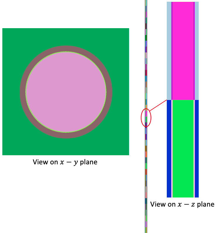
Figure 2: OpenMC geometry colored by cell ID shown on the - and - planes
The top and bottom of the pincell are vacuum boundaries. The four lateral faces of the pincell are reflective. Because we are not filling any universes with other universes or lattices, all of the cells in this problem are at the highest level of the geometry - i.e. the root universe.
We use a linear-linear stochastic interpolation between the two cross section data sets nearest to the imposed temperature by setting the method parameter on settings.temperature to interpolation. Finally, when OpenMC is initialized, cross section data is only loaded for a range of temperatures to save on memory usage; this range is specified with the temperature range element. You should set the range to be larger than the temperature range you expect in your coupled multiphysics problem - otherwise, you will encounter a runtime error that data is not available at the requested temperatures.
Because OpenMC runs at the end of each timestep, the initial fluid temperature is set to 280°C. And as there is no density feedback in this example, the densities initially imposed in the OpenMC model remain fixed at the values set in the OpenMC input files.
To generate the XML files needed to run OpenMC, you can run the following:
or simply use the XML files checked in to the tutorials/lwr_solid directory.
Multiphysics Coupling
In this section, OpenMC and MOOSE are coupled for heat source and temperature feedback for an LWR pincell. The following sub-sections describe these files.
Solid Input Files
The solid phase is solved with the MOOSE heat transfer module, and is described in the solid.i input. The solid mesh is created using mesh generators in the mesh.i input:
We generate the mesh by running cardinal-opt -i mesh.i --mesh-only to create the mesh_in.e file, which we then use in the solid input file.
OpenMC always has geometries set up in length units of centimeters. However, MOOSE is dimension-agnostic, and the same physics model can be set up in any length unit provided proper scalings are applied to material properties, source terms, and the mesh. In this example, we set up the solid input file in length units of centimeters.
The heat transfer module will solve for temperature, which we define as a nonlinear variable and apply a simple uniform initial condition.
(tutorials/lwr_solid/solid.i)The Transfer system in MOOSE is used to communicate variables across applications; a heat source will be computed by OpenMC and applied as a source term in MOOSE. In the opposite direction, MOOSE will compute a temperature that will be applied to the OpenMC geometry. Because we already solve for temperature, we simply need to add an auxiliary variable to receive the heat source from OpenMC.
(tutorials/lwr_solid/solid.i)The governing equation solved by MOOSE is specified in the [Kernels] block with the HeatConduction and CoupledForce kernels. The heat source provided by OpenMC is given by the receiver heat_source auxiliary variable.
We also set thermal conductivity values in the pellet and clad. Constant values are used for simplicity.
(tutorials/lwr_solid/solid.i)Next, the boundary conditions on the solid are applied, including the thermal contact model between the pellet and the clad.
(tutorials/lwr_solid/solid.i)In this example, the overall calculation workflow is as follows:
Run MOOSE heat conduction with a given power distribution from OpenMC.
Send temperature to OpenMC by modifying the temperature of OpenMC cells. A volume average is performed over all the MOOSE elements that mapped to a particular OpenMC cell.
Run OpenMC with an updated temperature distribution.
Extract the kappa-fission distribution (the recoverable fission energy) computed by OpenMC and map in the opposite direction from OpenMC cells to all the MOOSE elements that mapped to each cell.
The above sequence is repeated until desired convergence of the coupled domain is achieved. The MultiApps and Transfers blocks describe the interaction between Cardinal and MOOSE. The MOOSE heat conduction application is run as the main application, with OpenMC run as the sub-application. We specify that MOOSE will run first on each time step.
Two transfers are required to couple OpenMC and MOOSE for heat source and temperature feedback. The first is a transfer of heat source from Cardinal to MOOSE. The second is transfer of temperature from MOOSE to Cardinal.
(tutorials/lwr_solid/solid.i)For the heat source transfer from OpenMC, we ensure conservation by requiring that the integral of heat source computed by OpenMC (in the heat_source postprocessor) matches the integral of the heat source received by MOOSE (in the source_integral postprocessor). We also add a postprocessor to evaluate the maximum solid temperature.
Because we did not specify sub-cycling in the [MultiApps] block, this means that OpenMC will run for exactly the same number of time steps (but the actual time step size used by the OpenMC wrapping is of no consequence because OpenMC is run in -eigenvalue mode). By setting a fixed number of time steps, this example will simply run a fixed number of Picard iterations.
Neutronics Input Files
The neutronics physics is solved over the entire domain using OpenMC. The OpenMC wrapping is described in the openmc.i input file. We begin by defining a mesh on which OpenMC will receive temperature from the coupled MOOSE application, and on which OpenMC will write the fission heat source. In this example, we use exactly the same solid mesh as the coupled MOOSE application; this is not a requirement, and is relaxed in other tutorials.
Next, the Problem and Tallies blocks describe all objects necessary for the actual neutronics solve. To replace MOOSE finite element calculations with OpenMC particle transport calculations, the OpenMCCellAverageProblem class is used.
(tutorials/lwr_solid/openmc.i)For this example, we first start by specifying that we wish to add a CellTally in [Tallies]. The blocks are then used to indicate which OpenMC cells to add tallies to (as inferred from the mapping of MOOSE elements to OpenMC cells). If not specified, we add tallies to all OpenMC cells. But for this problem, we already know that the cladding doesn't have any fissile material, so we can save some effort with the tallies by skipping tallies in those regions by setting blocks to blocks 2 and 3. OpenMCCellAverageProblem will then take the information provided in the [Tallies] block and add the necessary OpenMC tally.
For this example, we specify the total fission power by which to normalize OpenMC's tally results (because OpenMC's tally results are in units of eV/source particle). Next, we indicate which blocks in the [Mesh] should be considered for temperature feedback using the temperature_blocks parameter. Here, we specify temperature feedback for the pellet (blocks 2 and 3) and the cladding (block 1). During the initialization, OpenMCCellAverageProblem will automatically map from MOOSE elements to OpenMC cells, and store which MOOSE elements are providing feedback. Then when temperature is sent into OpenMC, that mapping is used to compute a volume-average temperature to apply to each OpenMC cell. We specify the level in the geometry on which the cells exist. Because we don't have any lattices or filled universes in our OpenMC model, the cell level is zero.
Finally, we add a stochastic volume calculation in order to compare the actual volumes of OpenMC cells against the [Mesh] elements to which they map. A good mapping should show close agreement between these two values.
Next, we add a series of auxiliary variables for solution visualization (these are not requried for coupling). To help with understanding how Cardinal volume-averages temperature over the mesh, we add a CellTemperatureAux.
(tutorials/lwr_solid/openmc.i)Next, we specify an executioner and output settings. Even though OpenMC technically performs a criticality calculation (with no time dependence), we use the transient executioner so that if we wanted to run OpenMC more times than the coupled main application via subcycling, we would have a way to control that.
(tutorials/lwr_solid/openmc.i)Finally, we add a postprocessor to evaluate the total heat source computed by OpenMC. We also include a TallyRelativeError postprocessor to evaluate the maximum relative error of the cell tally and a third postprocessor to evaluate the maximum heat source.
(tutorials/lwr_solid/openmc.i)You will likely notice that many of the always-included MOOSE blocks are not present in the openmc.i input. OpenMCCellAverageProblem automatically adds the heat_source, temp, and density (if density is coupled to OpenMC) variables in the openmc.i input, so these will never appear in the OpenMC wrapper file explicitly. It is as if the following is included in the input file:
Execution and Postprocessing
To run the coupled calculation,
This will run both MOOSE and OpenMC with 2 MPI processes and 2 OpenMP threads per rank. To run the simulation faster, you can increase the parallel processes/threads, or simply decrease the number of particles used in OpenMC. When the simulation has completed, you will have created a number of different output files:
solid_out.e, an Exodus output with the solid mesh and solutionsolid_out_openmc0.e, an Exodus output with the OpenMC solution and the data that was ultimately transferred in/out of OpenMC
First, let's examine how the mapping between OpenMC and MOOSE was established. When we run with verbose = true, you will see the following mapping information displayed:
This shows the OpenMC cells mapped to the MOOSE elements. Because the gap between the pellet and cladding is un-meshed, the helium gap in the OpenMC model does not participate in coupling. The above message also shows the volume that each OpenMC cell maps to. Because there are no distributed cells in this problem, each cell only has a single instance. Since we added a stochastic volume calculation, the last column (Actual Vol) is populated with OpenMC's stochastic estimates for the cell volumes. You can increase the number of samples to drive the error lower to get more refined estimates of volumes.
Figure 3 shows the heat source computed by OpenMC (units of W/cm) and mapped to the MOOSE mesh; the block corresponding to the cladding is not shown. To the right is shown the heat source mapped along a line down the centerline of the rod. The heat source is slightly bottom-peaked due to the negative Doppler feedback from the fuel.
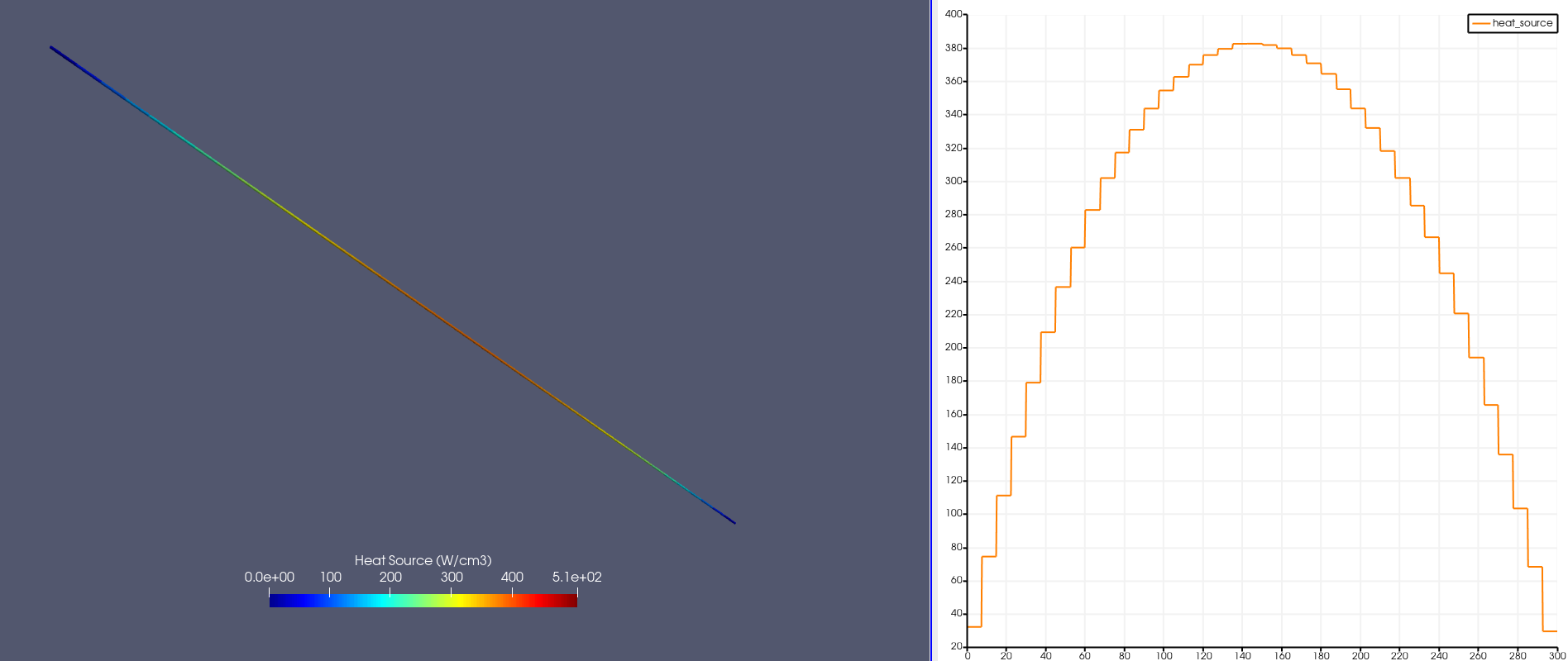
Figure 3: Heat source (W/cm) computed by OpenMC
Figure 4 shows the temperature computed by the MOOSE heat conduction module, while Figure 5 shows the temperature actually set in the OpenMC cells mapped to the MOOSE elements. Because a single cell was used to represent the cladding and fuel (at each axial layer), only one temperature is shown for the fuel and clad regions in the cell_temperature auxiliary variable. The temperatures set in OpenMC are volume averages of the temperature computed by MOOSE, i.e. the temperature shown in Figure 4. If you want to resolve the temperature with more detail in the OpenMC model, simply add OpenMC cells where finer feedback is desired.
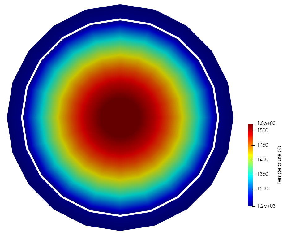
Figure 4: Temperature computed by MOOSE, on an slice
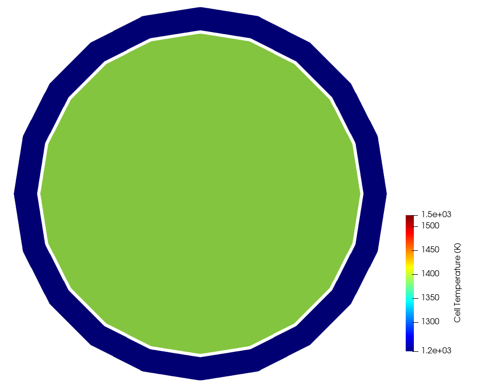
Figure 5: Temperature set in OpenMC cells (shown in terms of the [Mesh]), on the same slice shown in Figure 4
Adding Mesh Tallies
Next, we will replace the cell tallies with unstructured mesh tallies. That is, instead of setting tally_blocks and providing the MOOSE blocks to which the corresponding OpenMC cells should have tallies added, we will tally on an unstructured mesh. The inputs for this problem are largely the same as in Multiphysics Coupling ; the files are now solid_um.i and openmc_um.i. For the solid, we simply need to swap out the sub-application to point to a different input file.
Then, in openmc_um.i, we change the CellTally to a MeshTally. By default, OpenMC will then just tally directly on the MOOSE [Mesh] (though we could have specified a different mesh by providing a`mesh_template` file name).
By default, Cardinal will normalize the OpenMC fission energy tally according to a global tally over the entire OpenMC problem. When using mesh tallies on curvilinear surfaces, an unstructured mesh often cannot perfectly represent the domain. In this problem, for instance, the faceted nature of the pincell mesh means that a (small) amount of the fission energy is omitted in the tally because some regions of the OpenMC cell are outside any of the tally mesh elements (but still within the cylindrical pellet). In order to still obtain the specified power, we therefore change how the tallies are normalized. Instead of normalizing by a problem-wide tally (which includes the regions of the pellet that are outside the unstructured mesh but inside the pellet), we normalize instead by the sum of the mesh tally itself by setting normalize_by_global_tally to false. This ensures that the power we specify will be obtained when normalizing the OpenMC tally. In the limit of an extremely refined unstructured mesh, the error in normalizing by the global tally decreases to zero.
The mesh file we use for tallying is simply the mesh_in.e mesh we generated earlier with the mesh generators. Note that because the mesh in the [Mesh] block contains elements that correspond to the cladding, we will technically be tallying in cladding regions, even though there isn't a heat source there. Simply delete the cladding blocks in the mesh template if this is a concern.
There are several important limitations in the current implementation of mesh tallies in Cardinal - these will be relaxed in the future, but you must be aware of them with the current state of the repository. First, if the mesh provided by the mesh_template has elements, those elements must exactly match the first elements in the [Mesh]. The reason for this limitation is that the heat source tally is simply written to the corresponding mesh element in the [Mesh] by element index (as opposed to doing a nearest-element search). If the mesh in the [Mesh] block contains both solid and fluid elements, for instance, and you only want to tally on an unstructured mesh in the solid, all the solid elements in the [Mesh] should appear first in the total combined mesh. You can use a CombinerGenerator to achieve this if your fluid and solid meshes are saved in separate files or if you use separate mesh generators for the phases. We have checks in place to make sure you don't inadvertently bypass this requirement.
As some of the mesh tally bins are quite small, first increase the number of inactive batches from 500 to 1000 and the number of total batches from 1500 to 10000. Instead of re-running the make_openmc_model.py script, we can directly control these settings in the MOOSE-wrapped input file with the particles, inactive_batches, and batches parameters. Then, to run the input using mesh tallies, use:
To make the runtime faster, you can decrease the number of particles (though the heat source will have higher statistical noise). Figure 6 shows the unstructured mesh heat source computed by OpenMC; the clad region is shown as solid gray. You can see the "rim effect" common in LWR fuels, where the highest power is observed near the very edge of the fuel pellet. Because the tally bins are quite small, further increases in the total number of particles simulated will reduce the azimuthal asymmetry in the tally results in this azimuthally-symmetric geometry.
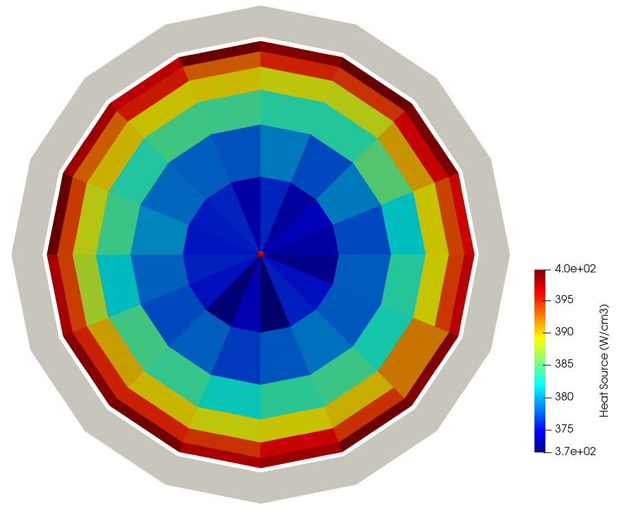
Figure 6: Unstructured mesh heat source computed by OpenMC, shown on the midplane of the pincell, with 20000 particles per batch, 1000 inactive batches, and 10000 total batches
Note that adding unstructured mesh tallies only affects how the heat source is measured in OpenMC - the use of unstructured mesh tallies has no bearing on the temperature and density resolution going into OpenMC. For this example, the temperature will have the same resolution as shown in Figure 5, albeit with slightly different values because the use of unstructured mesh tallies changes the coupled solution due to the different resolution of the heat source.