DAGMC Tokamak
In this tutorial, you will learn how to:
Export DAGMC models from Coreform Cubit
Couple CAD Monte Carlo models via temperature and heat source feedback to MOOSE
Use on-the-fly geometry regeneration to resolve temperature/density feedback in OpenMC
To access this tutorial,
cd cardinal/tutorials/tokamak
This tutorial also requires you to download some mesh files from Box. Please download the files from the tokamak folder here and place these files within tutorials/tokamak.
To run this tutorial, you need to have built Cardinal with DAGMC support enabled, by setting export ENABLE_DAGMC=true.
Geometry and Computational Models
This model consists of a 360-degree model of a tokamak, built using capabilities in Paramak. To further simplify the details in order to be suitable for a tutorial, the domain only consists of a tungsten first wall, homogenized multiplier and breeder layers, enclosed in a vacuum vessel. A simplified divertor component is also included. An image of an azimuthal slice of the CAD geometry is shown in Figure 1.
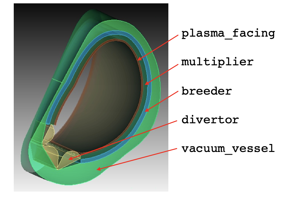
Figure 1: OpenMC DAGMC geometry colored by material; the names shown on the right correspond to the subdomain names
From Paramak, a STEP file is generated which can then be imported into Coreform Cubit. From within Coreform Cubit, we write a journal file (which can be "played" within the GUI) in order to assign materials, subdomain names, and boundary conditions. One notable difference from how we use DAGMC within Cardinal is the generation of two different meshes:
A mesh on which to solve the heat conduction problem, as well as to read/write data coupled in/out of OpenMC (
tokamak.e). This mesh is generated in units of meters.A triangulated surface mesh for transporting particles within OpenMC. This mesh is generated in units of centimeters.
#!python

# Path to the tutorials directory on your computer, if you want to run this script
directory = '/home/ajnovak2/cardinal/tutorials'

cubit.cmd("import step '" + directory + "/tokamak/iter05.step' heal no_names")

# simplify the CAD model for the sake of the tutorial, leaving only the first wall,
# multiplier, breeder, divertor, and vacuum vessel. These components are also
# represented as simple homogenized materials.
cubit.cmd("delete volume 2 3 4 5 6 7 8 9 10 11 12 13 15")
cubit.cmd("delete volume 1")

cubit.cmd("imprint volume all")
cubit.cmd("merge volume all")
cubit.cmd("compress all")

# sweep the geometry into 3D
cubit.cmd("sweep surface  2 zaxis angle 360 merge")
cubit.cmd("sweep surface 15 zaxis angle 360 merge")
cubit.cmd("sweep surface 18 zaxis angle 360 merge")
cubit.cmd("sweep surface 22 zaxis angle 360 merge")
cubit.cmd("sweep surface 37 zaxis angle 360 merge")

cubit.cmd("imprint volume all")
cubit.cmd("merge volume all")
cubit.cmd("compress all")

# these surfaces are next to one another, but one of them is very narrow
# so Cubit will try to generate tiny elements by default. Here, we composite the
# two surfaces into a new virtual surface, keeping the geometry unchanged, so that
# meshing treats both surfaces as a single unit
cubit.cmd("composite create surface 57 58 keep angle 15")

# create material tags that we will use to assign to the volumes
cubit.cmd("create material 'pf' property_group 'CUBIT-ABAQUS'")
cubit.cmd("create material 'multiplier' property_group 'CUBIT-ABAQUS'")
cubit.cmd("create material 'breeder' property_group 'CUBIT-ABAQUS'")
cubit.cmd("create material 'ss316' property_group 'CUBIT-ABAQUS'")

# add the volumes to blocks and give them names
cubit.cmd("block 1 add volume 1")
cubit.cmd("block 1 name 'plasma_facing'")
cubit.cmd("block 2 add volume 2")
cubit.cmd("block 2 name 'multiplier'")
cubit.cmd("block 3 add volume 3")
cubit.cmd("block 3 name 'breeder'")
cubit.cmd("block 4 add volume 4")
cubit.cmd("block 4 name 'divertor'")
cubit.cmd("block 5 add volume 5")
cubit.cmd("block 5 name 'vacuum_vessel'")

# assign the material tags to the corresponding blocks
cubit.cmd("block 1 material 'pf'")
cubit.cmd("block 2 material 'multiplier'")
cubit.cmd("block 3 material 'breeder'")
cubit.cmd("block 4 material 'pf'")
cubit.cmd("block 5 material 'ss316'")

cubit.cmd("volume all scheme tetmesh")
cubit.cmd("volume all size auto factor 5")
cubit.cmd("mesh volume all")

# export a volume mesh for the heat transfer solver and for mapping data in Cardinal.
# convert into meters before doing so, then back into centimeters (what DAGMC needs)
cubit.cmd("body all scale 0.01")
cubit.cmd("export Genesis '" + directory + "/tokamak/tokamak.e' dimension 3 overwrite")
cubit.cmd("body all scale 100.0")

# create a graveyard enclosing the domain to apply the vacuum boundary condition,
# as well as to obtain a surface on which we can set the reflective condition
# on the faces of the tokamak which are sliced
cubit.cmd("brick x 2010 y 2010 z 1140")
cubit.cmd("brick x 2100 y 2100 z 1180")
cubit.cmd("subtract body 6 from body 7")
cubit.cmd("block 8 add volume 8")
cubit.cmd("block 8 name 'graveyard'")
cubit.cmd("create material 'graveyard' property_group 'CUBIT-ABAQUS'")
cubit.cmd("block 8 material 'graveyard'")

# mesh the enclosing volumes using surface meshes
cubit.cmd("set trimesher coarse on ratio 100 angle 5")
cubit.cmd("surface all scheme trimesh")
cubit.cmd("volume 8 scheme tetmesh")
cubit.cmd("volume 8 size auto factor 10")
cubit.cmd("mesh volume 8")
After running the journal file, click "File -> Export -> DAGMC" in order to generate the tokamak.h5m file. Alternatively, you can download the mesh file and corresponding .h5m file from Box.
Paramak can provide a DAGMC geometry file to run OpenMC directly on. The reason only a STEP file was generated from Paramak, was to edit the CAD geometry to add multilayers for (tungsten first wall, multiplier, and breeder) and prepare the geometry to generate a volumetric mesh. The DAGMC h5m file was then exported from Cubit to match the final geometry which the volumetric mesh was generated from such that OpenMC cells are mapped correctly to MOOSE mesh elements. ### MOOSE Heat Conduction Model
The MOOSE heat transfer module is used to solve for steady-state heat conduction,
(1)
where is the solid thermal conductivity, is the solid temperature, and is a volumetric heat source in the solid.
Figure 2 shows a wedge of the 360-degree solid mesh.
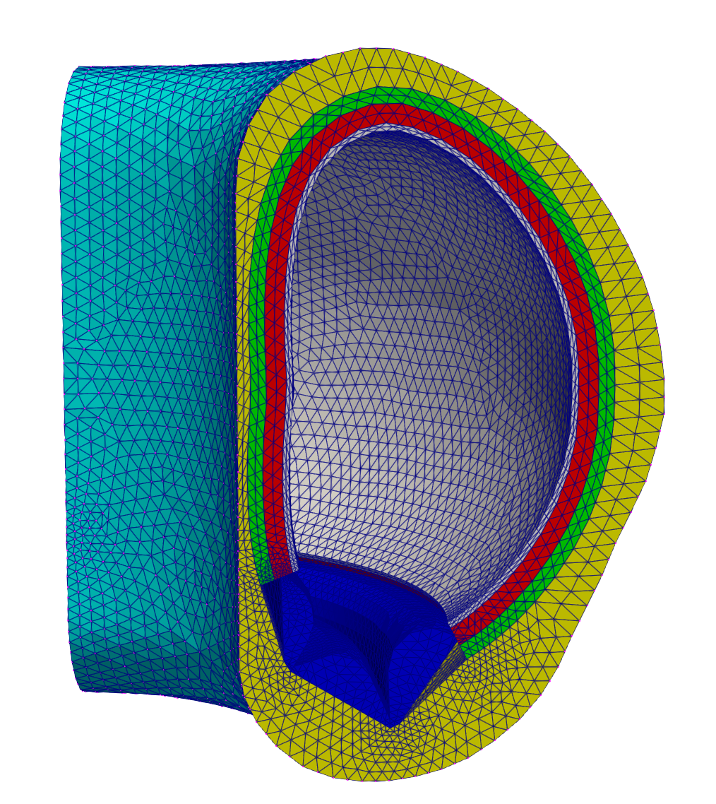
Figure 2: Mesh for the heat conduction problem; colors correspond to different subdomains
For simplicity, all regions will be modeled as purely conducting (no advection). This is a significant simplification over a realistic fusion device, and therefore the results obtained in this tutorial should not be taken as representative of a realistic device. However, for the purposes of a tutorial. there is minimal differences to establishing multiphysics feedback to OpenMC when adding a fluid solver. Other tutorials which apply density feedback, in addition to temperature feedback, can be found here and here.
To approximate some cooling in the breeder and divertor, we apply a uniform heat sink kernel. The magnitude of this heat sink is automatically computed in-line to obtain an approximate energy balance, by evaluating the difference in the heat deposition and heat flux on the vacuum vessel outer wall, divided by the volume in which the cooling is to be applied.
The boundary conditions applied to the heat conduction model are also highly simplified. On the exterior of the vacuum vessel, the temperature is set to a Dirichlet condition of 800 K. On all other sidesets, the boundary is assumed insulated.
OpenMC Model
The OpenMC model is built using DAGMC. Particles move through space with surface-to-surface tracking between triangle surface meshes. Cells are the regions of space enclosed by these surfaces. After building the DAGMC model with Cubit, we set up the OpenMC input files using the Python API. First, we define materials, then fetch the geometry from the DAGMC geometry file (tokamak.h5m). Then, we set up the settings, for numbers of batches and particles, and how we would like to have temperature feedback applied to OpenMC. The neutron source is set to a simple ring source, though more realistic fusion sources can be obtained accounting for the plasma parameters, such as some approximate pre-built sources here.
import openmc
import math

# define OpenMC materials; the names should match the names assigned to the blocks
# in the "block <n> material <name>" lines in the journal file

model = openmc.Model()

pf = openmc.Material(name="pf")
pf.set_density('g/cc', 19.30)
pf.add_element('W', 1.0)

ss316 = openmc.Material(name="ss316")
ss316.add_element('C', 0.0003, 'wo')
ss316.add_element('Mn', 0.02, 'wo')
ss316.add_element('Si', 0.01, 'wo')
ss316.add_element('P', 0.0005, 'wo')
ss316.add_element('S', 0.0002, 'wo')
ss316.add_element('Cr', 0.185, 'wo')
ss316.add_element('Mo', 0.025, 'wo')
ss316.add_element('Ni', 0.13, 'wo')
ss316.add_element('Fe', 0.629, 'wo')
ss316.set_density("g/cm3", 8.0)

eurofer = openmc.Material(name="eurofer")
eurofer.add_element('Fe', 0.011   , 'wo')
eurofer.add_element('Al', 0.002   , 'wo')
eurofer.add_element('As', 0.0002  , 'wo')
eurofer.add_element('B', 0.0012  , 'wo')
eurofer.add_element('C', 0.0005  , 'wo')
eurofer.add_element('Co', 0.0005  , 'wo')
eurofer.add_element('Cr', 0.0005  , 'wo')
eurofer.add_element('Cu', 0.00005 , 'wo')
eurofer.add_element('Mn', 0.00005 , 'wo')
eurofer.add_element('Mo', 0.0001  , 'wo')
eurofer.add_element('N', 0.0001  , 'wo')
eurofer.add_element('Nb', 0.00005 , 'wo')
eurofer.add_element('Ni', 0.0003  , 'wo')
eurofer.add_element('O', 0.00005 , 'wo')
eurofer.add_element('P', 0.004   , 'wo')
eurofer.add_element('S', 0.0001  , 'wo')
eurofer.add_element('Sb', 0.09    , 'wo')
eurofer.add_element('Sn', 0.0001  , 'wo')
eurofer.add_element('Si', 0.0011  , 'wo')
eurofer.add_element('Ta', 0.00002 , 'wo')
eurofer.add_element('Ti', 0.0005  , 'wo')
eurofer.add_element('V', 0       , 'wo')
eurofer.add_element('W', 0.0001  , 'wo')
eurofer.add_element('Zr', 0.88698 , 'wo')
eurofer.set_density("g/cm3", 7.798)

beryllium = openmc.Material(name="beryllium")
beryllium.add_element('Be', 1.0)
beryllium.set_density("g/cm3", 1.85)

Li4SiO4 = openmc.Material(name="Li4SiO4")
Li4SiO4.add_element('Li', 4.0)
Li4SiO4.add_element('Si', 1.0)
Li4SiO4.add_element('O', 4.0)
Li4SiO4.set_density("g/cm3", 2.39)

Helium = openmc.Material(name="Helium")
Helium.add_element('He', 1.0)
Helium.set_density("kg/m3", 0.166)

# define the breeder and multiplier as homogeneous mixtures of materials according to
# given atomic percents
Breeder = openmc.Material.mix_materials([eurofer, beryllium, Li4SiO4, Helium], [0.1, 0.37, 0.15, 0.38], 'ao',name="breeder")

Multiplier = openmc.Material.mix_materials([beryllium, Helium], [0.65, 0.35], 'ao', name="multiplier")

model.materials = openmc.Materials([pf, Breeder, Multiplier, ss316])

model.settings.dagmc = True
model.settings.photon_transport = True
model.settings.batches = 10
model.settings.particles = 10000
model.settings.run_mode = "fixed source"

model.settings.temperature = {'default': 800.0,
                              'method': 'interpolation',
                              'range': (294.0, 3000.0),
                              'tolerance': 1000.0}

# define the neutron source
source = openmc.IndependentSource()

r = openmc.stats.PowerLaw(600, 700, 1.0)
phi = openmc.stats.Uniform(0.0, 2*math.pi)
z = openmc.stats.Discrete([0,], [1.0,])
spatial_dist = openmc.stats.CylindricalIndependent(r, phi, z)

source.angle = openmc.stats.Isotropic()
source.energy = openmc.stats.Discrete([14.08e6], [1.0])
source.space=spatial_dist
model.settings.source = source

dagmc_univ = openmc.DAGMCUniverse(filename='tokamak.h5m')
model.geometry = openmc.Geometry(root=dagmc_univ)

model.export_to_xml()
To generate the XML files needed to run OpenMC, you can run the following:
python model.py
or simply use the XML files checked in to the tutorials/tokamak directory.
Multiphysics Coupling
In this section, OpenMC and MOOSE are coupled for heat source and temperature feedback for a tokamak. The following sub-sections describe these files.
Heat Conduction Files
The thermal physics is solved with the MOOSE heat transfer module, and is described in the solid.i input. The solid mesh is loaded from a file. Our Cubit mesh did not have any sidesets yet, so we add a sideset around the outside of the vacuum_vessel subdomain in order to later apply a boundary condition.
[Mesh<<<{"href": "../syntax/Mesh/index.html"}>>>]
  [file]
    type = FileMeshGenerator<<<{"description": "Read a mesh from a file.", "href": "../source/meshgenerators/FileMeshGenerator.html"}>>>
    file<<<{"description": "The filename to read."}>>> = tokamak.e
  []
  [add_outer_sideset]
    type = SideSetsAroundSubdomainGenerator<<<{"description": "Adds element faces that are on the exterior of the given block to the sidesets specified", "href": "../source/meshgenerators/SideSetsAroundSubdomainGenerator.html"}>>>
    input<<<{"description": "The mesh we want to modify"}>>> = file
    new_boundary<<<{"description": "The list of boundary names to create on the supplied subdomain"}>>> = 'outside'
    block<<<{"description": "The blocks around which to create sidesets"}>>> = 'vacuum_vessel'
  []
[]The heat transfer module will solve for temperature, with the heat equation. The variables, kernels, thermal conductivities, and boundary conditions are shown below.
[Variables<<<{"href": "../syntax/Variables/index.html"}>>>]
  [temp]
    initial_condition<<<{"description": "Specifies a constant initial condition for this variable"}>>> = 800.0
  []
[]

[AuxVariables<<<{"href": "../syntax/AuxVariables/index.html"}>>>]
  [heat_source]
    family<<<{"description": "Specifies the family of FE shape functions to use for this variable"}>>> = MONOMIAL
    order<<<{"description": "Specifies the order of the FE shape function to use for this variable (additional orders not listed are allowed)"}>>> = CONSTANT
  []
  [heat_removed_density]
    family<<<{"description": "Specifies the family of FE shape functions to use for this variable"}>>> = MONOMIAL
    order<<<{"description": "Specifies the order of the FE shape function to use for this variable (additional orders not listed are allowed)"}>>> = CONSTANT
    block = 'breeder divertor'
    initial_condition<<<{"description": "Specifies a constant initial condition for this variable"}>>> = -5000
  []
[]

[AuxKernels<<<{"href": "../syntax/AuxKernels/index.html"}>>>]
  [heat_removed]
    type = FunctionAux<<<{"description": "Auxiliary Kernel that creates and updates a field variable by sampling a function through space and time.", "href": "../source/auxkernels/FunctionAux.html"}>>>
    function<<<{"description": "The function to use as the value"}>>> = removal
    variable<<<{"description": "The name of the variable that this object applies to"}>>> = heat_removed_density
  []
[]

[Functions<<<{"href": "../syntax/Functions/index.html"}>>>]
  [removal]
    type = ParsedFunction<<<{"description": "Function created by parsing a string", "href": "../source/functions/MooseParsedFunction.html"}>>>
    expression<<<{"description": "The user defined function."}>>> = '-to_be_removed / volume'
    symbol_names<<<{"description": "Symbols (excluding t,x,y,z) that are bound to the values provided by the corresponding items in the symbol_values vector."}>>> = 'to_be_removed volume'
    symbol_values<<<{"description": "Constant numeric values, postprocessor names, function names, and scalar variables corresponding to the symbols in symbol_names."}>>> = 'to_be_removed volume'
  []
[]

[Kernels<<<{"href": "../syntax/Kernels/index.html"}>>>]
  [hc]
    type = HeatConduction<<<{"description": "Diffusive heat conduction term $-\\nabla\\cdot(k\\nabla T)$ of the thermal energy conservation equation", "href": "../source/kernels/HeatConduction.html"}>>>
    variable<<<{"description": "The name of the variable that this residual object operates on"}>>> = temp
  []
  [heat]
    type = CoupledForce<<<{"description": "Implements a source term proportional to the value of a coupled variable. Weak form: $(\\psi_i, -\\sigma v)$.", "href": "../source/kernels/CoupledForce.html"}>>>
    variable<<<{"description": "The name of the variable that this residual object operates on"}>>> = temp
    v<<<{"description": "The coupled variable which provides the force"}>>> = heat_source
  []
  [cooling]
    type = CoupledForce<<<{"description": "Implements a source term proportional to the value of a coupled variable. Weak form: $(\\psi_i, -\\sigma v)$.", "href": "../source/kernels/CoupledForce.html"}>>>
    variable<<<{"description": "The name of the variable that this residual object operates on"}>>> = temp
    block<<<{"description": "The list of blocks (ids or names) that this object will be applied"}>>> = 'breeder divertor'
    v<<<{"description": "The coupled variable which provides the force"}>>> = heat_removed_density
  []
[]

[BCs<<<{"href": "../syntax/BCs/index.html"}>>>]
  [surface]
    type = DirichletBC<<<{"description": "Imposes the essential boundary condition $u=g$, where $g$ is a constant, controllable value.", "href": "../source/bcs/DirichletBC.html"}>>>
    variable<<<{"description": "The name of the variable that this residual object operates on"}>>> = temp
    boundary<<<{"description": "The list of boundary IDs from the mesh where this object applies"}>>> = 'outside'
    value<<<{"description": "Value of the BC"}>>> = 800.0
  []
[]

[Materials<<<{"href": "../syntax/Materials/index.html"}>>>]
  [k_1]
    type = GenericConstantMaterial<<<{"description": "Declares material properties based on names and values prescribed by input parameters.", "href": "../source/materials/GenericConstantMaterial.html"}>>>
    prop_values<<<{"description": "The values associated with the named properties"}>>> = '175'
    prop_names<<<{"description": "The names of the properties this material will have"}>>> = 'thermal_conductivity'
    block<<<{"description": "The list of blocks (ids or names) that this object will be applied"}>>> = 'plasma_facing divertor'
  []
  [k_2]
    type = GenericConstantMaterial<<<{"description": "Declares material properties based on names and values prescribed by input parameters.", "href": "../source/materials/GenericConstantMaterial.html"}>>>
    prop_values<<<{"description": "The values associated with the named properties"}>>> = '16.3'
    prop_names<<<{"description": "The names of the properties this material will have"}>>> = 'thermal_conductivity'
    block<<<{"description": "The list of blocks (ids or names) that this object will be applied"}>>> = 'vacuum_vessel'
  []
  [k_3]
    type = GenericConstantMaterial<<<{"description": "Declares material properties based on names and values prescribed by input parameters.", "href": "../source/materials/GenericConstantMaterial.html"}>>>
    prop_values<<<{"description": "The values associated with the named properties"}>>> = '20.0'
    prop_names<<<{"description": "The names of the properties this material will have"}>>> = 'thermal_conductivity'
    block<<<{"description": "The list of blocks (ids or names) that this object will be applied"}>>> = 'multiplier breeder'
  []
[]The MultiApps and Transfers blocks describe the interaction between Cardinal and MOOSE. The MOOSE heat conduction application is run as the main application, with OpenMC run as the sub-application. We specify that MOOSE will run first on each time step.
Two transfers are required to couple OpenMC and MOOSE for heat source and temperature feedback. The first is a transfer of heat source from Cardinal to MOOSE. The second is transfer of temperature from MOOSE to Cardinal.
[MultiApps<<<{"href": "../syntax/MultiApps/index.html"}>>>]
  [openmc]
    type = TransientMultiApp<<<{"description": "MultiApp for performing coupled simulations with the parent and sub-application both progressing in time.", "href": "../source/multiapps/TransientMultiApp.html"}>>>
    input_files<<<{"description": "The input file for each App.  If this parameter only contains one input file it will be used for all of the Apps.  When using 'positions_from_file' it is also admissable to provide one input_file per file."}>>> = 'openmc.i'
    execute_on<<<{"description": "The list of flag(s) indicating when this object should be executed. For a description of each flag, see https://mooseframework.inl.gov/source/interfaces/SetupInterface.html."}>>> = timestep_begin
  []
[]

[Transfers<<<{"href": "../syntax/Transfers/index.html"}>>>]
  [heat_source_from_openmc]
    type = MultiAppGeneralFieldShapeEvaluationTransfer<<<{"description": "Transfers field data at the MultiApp position using the finite element shape functions from the origin application.", "href": "../source/transfers/MultiAppGeneralFieldShapeEvaluationTransfer.html"}>>>
    from_multi_app<<<{"description": "The name of the MultiApp to receive data from"}>>> = openmc
    variable<<<{"description": "The auxiliary variable to store the transferred values in."}>>> = heat_source
    source_variable<<<{"description": "The variable to transfer from."}>>> = heating_local
    from_postprocessors_to_be_preserved<<<{"description": "The name of the Postprocessor in the from-app to evaluate an adjusting factor."}>>> = heating
    to_postprocessors_to_be_preserved<<<{"description": "The name of the Postprocessor in the to-app to evaluate an adjusting factor."}>>> = source_integral
  []
  [temp_to_openmc]
    type = MultiAppGeneralFieldShapeEvaluationTransfer<<<{"description": "Transfers field data at the MultiApp position using the finite element shape functions from the origin application.", "href": "../source/transfers/MultiAppGeneralFieldShapeEvaluationTransfer.html"}>>>
    to_multi_app<<<{"description": "The name of the MultiApp to transfer the data to"}>>> = openmc
    variable<<<{"description": "The auxiliary variable to store the transferred values in."}>>> = temp
    source_variable<<<{"description": "The variable to transfer from."}>>> = temp
  []
[]For the heat source transfer from OpenMC, we ensure conservation by requiring that the integral of heat source computed by OpenMC (in the heating postprocessor) matches the integral of the heat source received by MOOSE (in the source_integral postprocessor).
Additional postprocessors are added to compute several integrals in-line in order to apply the heat sink term to approximate an energy balance. The total heat which must be removed by the heat sink added in the breeder and divertor will be equal to the magnitude of the nuclear heating, minus any heat flux from the vacuum vessel surface. This quantity is computed in the to_be_removed postprocessor. This power, divided by the volume of the breeder and divertor (the volume postprocessor), is then applied to the heat_removed_density auxvariable.
[Postprocessors<<<{"href": "../syntax/Postprocessors/index.html"}>>>]
  [source_integral]
    type = ElementIntegralVariablePostprocessor<<<{"description": "Computes a volume integral of the specified variable", "href": "../source/postprocessors/ElementIntegralVariablePostprocessor.html"}>>>
    variable<<<{"description": "The name of the variable that this object operates on"}>>> = heat_source
    execute_on<<<{"description": "The list of flag(s) indicating when this object should be executed. For a description of each flag, see https://mooseframework.inl.gov/source/interfaces/SetupInterface.html."}>>> = transfer
  []
  [removal_integral]
    type = ElementIntegralVariablePostprocessor<<<{"description": "Computes a volume integral of the specified variable", "href": "../source/postprocessors/ElementIntegralVariablePostprocessor.html"}>>>
    variable<<<{"description": "The name of the variable that this object operates on"}>>> = heat_removed_density
    execute_on<<<{"description": "The list of flag(s) indicating when this object should be executed. For a description of each flag, see https://mooseframework.inl.gov/source/interfaces/SetupInterface.html."}>>> = timestep_end
    block<<<{"description": "The list of blocks (ids or names) that this object will be applied"}>>> = 'breeder divertor'
  []
  [heat_loss_vessel]
    type = SideDiffusiveFluxIntegral<<<{"description": "Computes the integral of the diffusive flux over the specified boundary", "href": "../source/postprocessors/SideDiffusiveFluxIntegral.html"}>>>
    variable<<<{"description": "The name of the variable which this postprocessor integrates"}>>> = temp
    diffusivity<<<{"description": "The name of the diffusivity material property that will be used in the flux computation. This must be provided if the variable is of finite element type"}>>> = thermal_conductivity
    boundary<<<{"description": "The list of boundary IDs from the mesh where this object applies"}>>> = 'outside'
  []
  [energy_balance]
    type = ParsedPostprocessor<<<{"description": "Computes a parsed expression with post-processors", "href": "../source/postprocessors/ParsedPostprocessor.html"}>>>
    expression<<<{"description": "function expression"}>>> = 'source_integral + removal_integral - heat_loss_vessel'
    pp_names<<<{"description": "Post-processors arguments"}>>> = 'source_integral removal_integral heat_loss_vessel'
  []

  # determine what to set the heat removal to in order to obtain an energy balance
  [to_be_removed]
    type = ParsedPostprocessor<<<{"description": "Computes a parsed expression with post-processors", "href": "../source/postprocessors/ParsedPostprocessor.html"}>>>
    expression<<<{"description": "function expression"}>>> = 'source_integral - heat_loss_vessel'
    pp_names<<<{"description": "Post-processors arguments"}>>> = 'source_integral heat_loss_vessel'
  []
  [volume]
    type = VolumePostprocessor<<<{"description": "Computes the volume of a specified block", "href": "../source/postprocessors/VolumePostprocessor.html"}>>>
    block<<<{"description": "The list of blocks (ids or names) that this object will be applied"}>>> = 'breeder divertor'
    execute_on<<<{"description": "The list of flag(s) indicating when this object should be executed. For a description of each flag, see https://mooseframework.inl.gov/source/interfaces/SetupInterface.html."}>>> = 'initial'
  []
[]Because we did not specify sub-cycling in the [MultiApps] block, this means that OpenMC will run for exactly the same number of steps (i.e., Picard iterations).
[Executioner<<<{"href": "../syntax/Executioner/index.html"}>>>]
  type = Transient

  petsc_options_value = 'hypre boomeramg'
  petsc_options_iname = '-pc_type -pc_hypre_type'

  steady_state_detection = true

  # you want to make this tighter for production runs
  steady_state_tolerance = 2e-2
[]

[Outputs<<<{"href": "../syntax/Outputs/index.html"}>>>]
  exodus<<<{"description": "Output the results using the default settings for Exodus output."}>>> = true
  csv<<<{"description": "Output the scalar variable and postprocessors to a *.csv file using the default CSV output."}>>> = true
  hide<<<{"description": "A list of the variables and postprocessors that should NOT be output to the Exodus file (may include Variables, ScalarVariables, and Postprocessor names)."}>>> = 'to_be_removed volume'
[]Neutronics Input Files
The neutronics physics is solved over the entire domain using OpenMC. The OpenMC wrapping is described in the openmc.i input file. We begin by defining a mesh on which OpenMC will receive temperature from the coupled MOOSE application, and on which OpenMC will write the nuclear heating.
[Mesh<<<{"href": "../syntax/Mesh/index.html"}>>>]
  [file]
    type = FileMeshGenerator<<<{"description": "Read a mesh from a file.", "href": "../source/meshgenerators/FileMeshGenerator.html"}>>>
    file<<<{"description": "The filename to read."}>>> = tokamak.e
  []
[]Next, the Problem block describes all objects necessary for the actual physics solve. To replace MOOSE finite element calculations with OpenMC particle transport calculations, the OpenMCCellAverageProblem class is used.
[Problem<<<{"href": "../syntax/Problem/index.html"}>>>]
  type = OpenMCCellAverageProblem
  scaling = 100.0

  source_strength = 2e18

  cell_level = 0
  temperature_blocks = 'plasma_facing multiplier breeder divertor vacuum_vessel'

  # this is a low number of particles; you will want to increase in order to obtain
  # high-quality results
  first_iteration_particles = 1000
  relaxation = dufek_gudowski

  skinner = moab

  [Tallies<<<{"href": "../syntax/Problem/Tallies/index.html"}>>>]
    [tokamak]
      type = MeshTally<<<{"description": "A class which implements unstructured mesh tallies.", "href": "../source/tallies/MeshTally.html"}>>>
      mesh_template<<<{"description": "Mesh tally template for OpenMC when using mesh tallies; at present, this mesh must exactly match the mesh used in the [Mesh] block because a one-to-one copy is used to get OpenMC's tally results on the [Mesh]."}>>> = tokamak.e
      score<<<{"description": "Score(s) to use in the OpenMC tallies. If not specified, defaults to 'kappa_fission'"}>>> = 'heating_local H3_production'
      output<<<{"description": "UNRELAXED field(s) to output from OpenMC for each tally score. unrelaxed_tally_std_dev will write the standard deviation of each tally into auxiliary variables named *_std_dev. unrelaxed_tally_rel_error will write the relative standard deviation (unrelaxed_tally_std_dev / unrelaxed_tally) of each tally into auxiliary variables named *_rel_error. unrelaxed_tally will write the raw unrelaxed tally into auxiliary variables named *_raw (replace * with 'name')."}>>> = unrelaxed_tally_std_dev
    []
  []
[]For this example, we specify the total neutron source rate (neutrons/s) by which to normalize OpenMC's tally results (because OpenMC's heating tally results are in units of eV/source particle). Next, we indicate which blocks in the [Mesh] should be considered for temperature feedback using temperature_blocks. Here, we specify temperature feedback for all blocks in the mesh. During the initialization, OpenMCCellAverageProblem will automatically map from MOOSE elements to OpenMC cells, and store which MOOSE elements are providing temperature feedback. Then when temperature is sent into OpenMC, that mapping is used to compute a volume-average temperature to apply to each OpenMC cell.
This example uses mesh tallies, as indicated by the MeshTally in the Tallies block. In this example, we will tally on the same mesh given in the [Mesh] block. Finally, we specify the level in the geometry on which the cells exist. Because we don't have any lattices or filled universes in our OpenMC model, the cell level is zero.
It is common when performing multiphysics with Monte Carlo solvers to use relaxation schemes. Here, we use the Dufek-Gudowski scheme to slowly ramp up the number of particles used in each successive OpenMC solve.
On the first time step, our OpenMC model contains five cells (one large cell each to represent the entire first wall, multiplier, breeder, vacuum vessel, and divertor). Because OpenMC uses surface tracking, this means that multiphysics feedback would impose a significant constraint that the temperature and density of each of these regions would be homogeneous (constant). However, there will exist gradients in temperature and/or density in these components as computed by the thermal-fluid physics. In order to more finely capture these feedback effects, we add a MoabSkinner object in order to on-the-fly regenerated the OpenMC cells according to contours in temperature and/or density. Here, we will re-generate the Monte Carlo model to create new cells for every 50 K in temperature difference.
[UserObjects<<<{"href": "../syntax/UserObjects/index.html"}>>>]
  [moab]
    type = MoabSkinner<<<{"description": "Re-generate the OpenMC geometry on-the-fly according to changes in the mesh geometry and/or contours in temperature and density", "href": "../source/userobjects/MoabSkinner.html"}>>>
    temperature_min<<<{"description": "Lower bound of temperature bins"}>>> = 0
    temperature_max<<<{"description": "Upper bound of temperature bins"}>>> = 2000
    n_temperature_bins<<<{"description": "Number of temperature bins"}>>> = 40
    temperature<<<{"description": "Temperature variable by which to bin elements"}>>> = temp
    build_graveyard<<<{"description": "Whether to build a graveyard around the geometry"}>>> = true
    output_skins<<<{"description": "Whether the skinned MOAB mesh (skins generated from the libMesh [Mesh]) should be written to a file. The files will be named moab_skins_<n>.h5m, where <n> is the time step index. You can then visualize these files by running 'mbconvert'."}>>> = true
  []
[]Next, we add a series of auxiliary variables for solution visualization (these are not requried for coupling). To help with understanding how the OpenMC model maps to the mesh in the [Mesh] block, we add auxiliary variables to visualize OpenMC's cell temperature (CellTemperatureAux). Cardinal will also automatically output a variable named cell_id (CellIDAux) and a variable named cell_instance ( CellInstanceAux) to show the spatial mapping.
[AuxVariables<<<{"href": "../syntax/AuxVariables/index.html"}>>>]
  [cell_temperature]
    family<<<{"description": "Specifies the family of FE shape functions to use for this variable"}>>> = MONOMIAL
    order<<<{"description": "Specifies the order of the FE shape function to use for this variable (additional orders not listed are allowed)"}>>> = CONSTANT
  []
[]

[AuxKernels<<<{"href": "../syntax/AuxKernels/index.html"}>>>]
  [cell_temperature]
    type = CellTemperatureAux<<<{"description": "OpenMC cell temperature (K), mapped to each MOOSE element", "href": "../source/auxkernels/CellTemperatureAux.html"}>>>
    variable<<<{"description": "The name of the variable that this object applies to"}>>> = cell_temperature
  []
[]Next, we specify an executioner and output settings. Even though OpenMC technically performs a fixed source calculation (with no time dependence), we use the transient executioner so that if we wanted to run OpenMC more times than the coupled main application via subcycling, we would have a way to control that.
[Executioner<<<{"href": "../syntax/Executioner/index.html"}>>>]
  type = Transient
[]

[Outputs<<<{"href": "../syntax/Outputs/index.html"}>>>]
  exodus<<<{"description": "Output the results using the default settings for Exodus output."}>>> = true
  csv<<<{"description": "Output the scalar variable and postprocessors to a *.csv file using the default CSV output."}>>> = true
[]Finally, we add a postprocessor to evaluate the total heat source computed by OpenMC and query other parts of the solution.
[Postprocessors<<<{"href": "../syntax/Postprocessors/index.html"}>>>]
  [heating]
    type = ElementIntegralVariablePostprocessor<<<{"description": "Computes a volume integral of the specified variable", "href": "../source/postprocessors/ElementIntegralVariablePostprocessor.html"}>>>
    variable<<<{"description": "The name of the variable that this object operates on"}>>> = heating_local
  []
  [tritium_production]
    type = ElementIntegralVariablePostprocessor<<<{"description": "Computes a volume integral of the specified variable", "href": "../source/postprocessors/ElementIntegralVariablePostprocessor.html"}>>>
    variable<<<{"description": "The name of the variable that this object operates on"}>>> = H3_production
  []
  [tritium_error]
    type = TallyRelativeError<<<{"description": "Maximum/minimum tally relative error", "href": "../source/postprocessors/TallyRelativeError.html"}>>>
    tally_score<<<{"description": "Score to report the relative error. If there is just a single score, this defaults to that value"}>>> = H3_production
    value_type<<<{"description": "Whether to give the maximum or minimum tally relative error"}>>> = average
  []
  [heating_error]
    type = TallyRelativeError<<<{"description": "Maximum/minimum tally relative error", "href": "../source/postprocessors/TallyRelativeError.html"}>>>
    tally_score<<<{"description": "Score to report the relative error. If there is just a single score, this defaults to that value"}>>> = heating_local
    value_type<<<{"description": "Whether to give the maximum or minimum tally relative error"}>>> = average
  []
[]Execution and Postprocessing
To run the coupled calculation,
mpiexec -np 2 cardinal-opt -i solid.i --n-threads=2
This will run both MOOSE and OpenMC with 2 MPI processes and 2 OpenMP threads per rank. To run the simulation faster, you can increase the parallel processes/threads, or simply decrease the number of particles used in OpenMC. When the simulation has completed, you will have created a number of different output files:
solid_out.e, an Exodus output with the solid mesh and solutionsolid_out_openmc0.e, an Exodus output with the OpenMC solution and the data that was ultimately transferred in/out of OpenMC
Figure 3 shows the heat source computed by OpenMC (units of W/cm) and mapped to the MOOSE mesh and the solid temperature computed by MOOSE, on the last Picard iteration. Note that these results are not necessarily intended to replicate a realistic tokamak, due to the highly simplified neutron source and lack of fluid flow cooling.
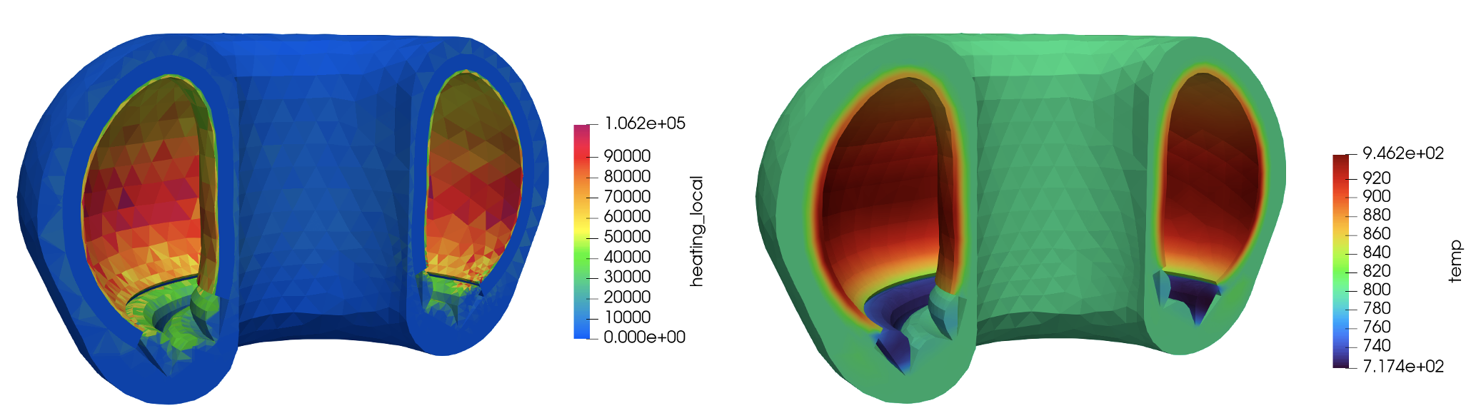
Figure 3: Heat source (W/cm) computed by OpenMC (left); MOOSE solid temperature (right)