Solid and Fluid Coupling of OpenMC and MOOSE

In this tutorial, you will learn how to:

Couple OpenMC to 2 separate MOOSE applications solving for the solid and fluid thermal-fluids
Couple OpenMC to mixed-dimension feedback with 3-D heat conduction and 1-D fluid flow
Establish coupling between OpenMC and MOOSE for nested universe OpenMC models
Apply homogenized temperature feedback to heterogeneous OpenMC cells

To access this tutorial:


cd cardinal/tutorials/gas_assembly

This tutorial also requires you to download an OpenMC XML file from Box. Please download the files from the gas_assembly folder here and place these files within the same directory structure in tutorials/gas_assembly.

In this tutorial, we couple OpenMC to the MOOSE heat transfer module and the Thermal Hydraulics Module (THM) , a set of 1-D systems-level thermal-hydraulics kernels. OpenMC will receive temperature feedback from both the MOOSE heat transfer module (for the solid regions) and from THM (for the fluid regions). Density feedback will be provided by THM for the fluid regions. This tutorial models a full-height TRISO-fueled prismatic gas reactor fuel assembly, and is an extension of an earlier tutorial which coupled OpenMC and MOOSE heat conduction (i.e. without an application providing fluid feedback) for a unit cell version of the same geometry. In this tutorial, we add fluid feedback and also describe several nuances associated with setting up feedback in OpenMC lattices.

This tutorial was developed with support from the NEAMS Thermal Fluids Center of Excellence. A paper Novak et al. (2021) describing the physics models and mesh refinement studies provides additional context beyond the scope of this tutorial.

Due to the tall height of the full assembly (about 6 meters), the converged results shown in Novak et al. (2021) and in the figures in this tutorial used a finer mesh and more particles than in the input files we set up for this tutorial - the input files in this tutorial still require parallel resources to run, but should be faster-running. Parameters that have been set to coarser values are noted where applicable.

Geometry and Computational Model

The geometry consists of a TRISO-fueled gas reactor assembly INL (2016). A top-down view of the geometry is shown in Figure 1. The assembly is a graphite prismatic hexagonal block with 108 helium coolant channels, 210 fuel compacts, and 6 poison compacts. Each fuel compact contains TRISO particles dispersed in a graphite matrix with a packing fraction of 15%. All channels and compacts are ordered in a triangular lattice with pitch $var element = document.getElementById("moose-equation-b54687c6-c568-4303-87fe-dfdc5e1e8f29");katex.render("p_{cf}", element, {displayMode:false,throwOnError:false});$ . Due to irradiation- and temperature-induced swelling of graphite, small helium gaps exist between assemblies. In this tutorial, rather than explicitly model the inter-assembly flow, we treat the gap regions as solid graphite. There are also graphite reflectors above and below the assembly.

Figure 1: TRISO-fueled gas reactor fuel assembly

The TRISO particles use a conventional design that consists of a central fissile uranium oxycarbide kernel enclosed in a carbon buffer, an inner PyC layer, a silicon carbide layer, and finally an outer PyC layer. The geometric specifications for the assembly dimensions are shown in Figure 1, while dimensions for the TRISO particles are summarized in Table 1.

Table 1: Geometric specifications for the TRISO particles

Parameter	Value (cm)
TRISO kernel radius	214.85e-4
Buffer layer radius	314.85e-4
Inner PyC layer radius	354.85e-4
Silicon carbide layer radius	389.85e-4
Outer PyC layer radius	429.85e-4

Heat is produced in the TRISO particles to yield a total power of 16.7 MWth. This heat is removed by helium flowing downwards through the coolant channels with a total mass flowrate of 9.775 kg/s, which is assumed to be uniformly distributed among the coolant channels. The outlet pressure is 7.1 MPa.

Heat Conduction Model

The MOOSE heat transfer module is used to solve for steady-state heat conduction,

$(1)var element = document.getElementById("moose-equation-064c4464-691c-48e3-8fff-1a811eff04f8");katex.render(" -\\nabla\\cdot\\left(k_s\\nabla T_s\\right)=\\dot{q}_s", element, {displayMode:true,throwOnError:false});$

where $var element = document.getElementById("moose-equation-972f41d3-5af9-4d37-a7ab-826674da7c49");katex.render("k_s", element, {displayMode:false,throwOnError:false});$ is the solid thermal conductivity, $var element = document.getElementById("moose-equation-80c91cbf-31a4-4125-8653-b0d530181690");katex.render("T_s", element, {displayMode:false,throwOnError:false});$ is the solid temperature, and $var element = document.getElementById("moose-equation-e8a8f330-0f95-45eb-8203-1856f6561a48");katex.render("\\dot{q}_s", element, {displayMode:false,throwOnError:false});$ is a volumetric heat source in the solid.

To greatly reduce meshing requirements, the TRISO particles are homogenized into the compact regions by volume-averaging material properties. The solid mesh is shown in Figure 2. The only sideset in the domain is the coolant channel surface, which is named fluid_solid_interface. The solid geometry uses a length unit of meters. The solid mesh is created using the MOOSE reactor module Shemon et al. (2021), which provides easy-to-use mesh generators to programmatically construct reactor core meshes as building blocks of bundle and pincell meshes.

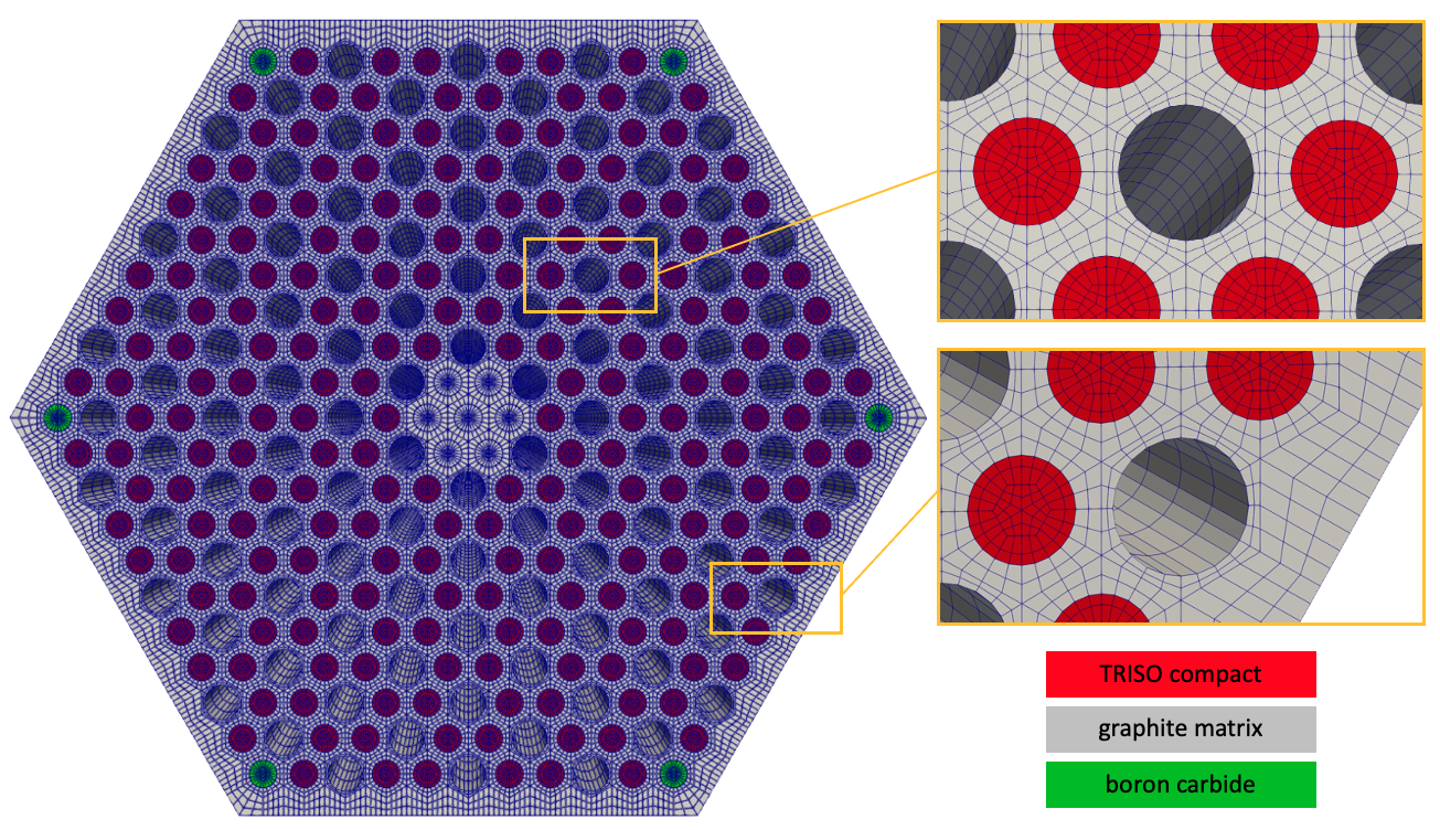
Figure 2: Converged mesh for the solid heat conduction model (with 300 axial layers); to make the tutorial run faster, our mesh will only use 100 axial layers

The file used to generate the solid mesh is shown below. The mesh is created by first building pincell meshes for a fuel pin, a coolant pin, a poison pin, and a graphite "pin" (to represent the central graphite region). The pin meshes are then combined together into a bundle pattern and extruded.

n_layers = 100    # number of axial extrusion layers; for the converged case,
                  # we set this to 300 to get a finer mesh

[GlobalParams]
  quad_center_elements = true
[]

[Mesh]
  [fuel_pin]
    type = PolygonConcentricCircleMeshGenerator
    num_sides = 6
    polygon_size = ${fparse fuel_to_coolant_distance / 2.0}
    ring_radii = '${fparse 0.8 * compact_diameter / 2.0} ${fparse compact_diameter / 2.0}'
    ring_intervals = '1 1'
    num_sectors_per_side = '4 4 4 4 4 4'
    ring_block_ids = '2 2'
    ring_block_names = 'compacts compacts'
    background_block_ids = '1'
    background_block_names = 'graphite'
    background_intervals = 2
  []
  [coolant_pin]
    type = PolygonConcentricCircleMeshGenerator
    num_sides = 6
    polygon_size = ${fparse fuel_to_coolant_distance / 2.0}
    ring_radii = '${fparse channel_diameter / 2.0}'
    ring_intervals = '2'
    num_sectors_per_side = '4 4 4 4 4 4'
    ring_block_ids = '101 101'
    ring_block_names = 'coolant coolant'
    background_block_ids = '1'
    background_block_names = 'graphite'
    interface_boundary_id_shift = 100
    create_inward_interface_boundaries = true
    background_intervals = 2
  []
  [poison_pin]
    type = PolygonConcentricCircleMeshGenerator
    num_sides = 6
    polygon_size = ${fparse fuel_to_coolant_distance / 2.0}
    ring_radii = '${fparse compact_diameter / 2.0}'
    ring_intervals = '2'
    num_sectors_per_side = '4 4 4 4 4 4'
    ring_block_ids = '4 4'
    ring_block_names = 'poison poison'
    background_block_ids = '1'
    background_block_names = 'graphite'
    background_intervals = 2
  []
  [graphite_pin]
    type = PolygonConcentricCircleMeshGenerator
    num_sides = 6
    polygon_size = ${fparse fuel_to_coolant_distance / 2.0}
    ring_radii = '${fparse compact_diameter / 2.0}'
    ring_intervals = '2'
    num_sectors_per_side = '4 4 4 4 4 4'
    ring_block_ids = '1 1'
    ring_block_names = 'graphite graphite'
    background_block_ids = '1'
    background_block_names = 'graphite'
  []
  [bundle]
    type = PatternedHexMeshGenerator
    inputs = 'fuel_pin coolant_pin poison_pin graphite_pin'
    hexagon_size = ${fparse bundle_flat_to_flat / 2.0 + bundle_gap_width / 2.0}
    pattern = '2 0 1 0 0 1 0 0 1 0 2;
              0 1 0 0 1 0 0 1 0 0 1 0;
             1 0 0 1 0 0 1 0 0 1 0 0 1;
            0 0 1 0 0 1 0 0 1 0 0 1 0 0;
           0 1 0 0 1 0 0 1 0 0 1 0 0 1 0;
          1 0 0 1 0 0 1 0 0 1 0 0 1 0 0 1;
         0 0 1 0 0 1 0 0 1 0 0 1 0 0 1 0 0;
        0 1 0 0 1 0 0 1 0 0 1 0 0 1 0 0 1 0;
       1 0 0 1 0 0 1 0 0 1 0 0 1 0 0 1 0 0 1;
      0 0 1 0 0 1 0 0 1 3 3 1 0 0 1 0 0 1 0 0;
     2 1 0 0 1 0 0 1 0 3 3 3 0 1 0 0 1 0 0 1 2;
      0 0 1 0 0 1 0 0 1 3 3 1 0 0 1 0 0 1 0 0;
       1 0 0 1 0 0 1 0 0 1 0 0 1 0 0 1 0 0 1;
        0 1 0 0 1 0 0 1 0 0 1 0 0 1 0 0 1 0;
         0 0 1 0 0 1 0 0 1 0 0 1 0 0 1 0 0;
          1 0 0 1 0 0 1 0 0 1 0 0 1 0 0 1;
           0 1 0 0 1 0 0 1 0 0 1 0 0 1 0;
            0 0 1 0 0 1 0 0 1 0 0 1 0 0;
             1 0 0 1 0 0 1 0 0 1 0 0 1;
              0 1 0 0 1 0 0 1 0 0 1 0;
               2 0 1 0 0 1 0 0 1 0 2'
    rotate_angle = 0

    background_block_id = '1'
  []
  [extrude]
    type = AdvancedExtruderGenerator
    input = bundle
    heights = ${height}
    num_layers = ${n_layers}
    direction = '0 0 1'
  []
  [delete_coolant]
    type = BlockDeletionGenerator
    input = extrude
    block = '101'
  []
  [rename_coolant_sideset]
    type = RenameBoundaryGenerator
    input = delete_coolant
    old_boundary = 102
    new_boundary = 'fluid_solid_interface'
  []

  construct_side_list_from_node_list = true
[]

# The following content is adding postprocessor(s) to check sideset areas.
# The reactor module is unfortunately quite brittle in its assignment of sideset
# IDs, so we want to be extra sure that any changes to sideset numbering are detected
# in our test suite.

You can create this mesh by running:


cardinal-opt -i common_input.i solid_mesh.i --mesh-only

which will create a mesh named solid_mesh_in.e. Note that the above command takes advantage of a MOOSE feature for combining input files together by placing some common parameters used by the other applications into a file named common_input.i.

The temperature on the fluid-solid interface is provided by Thermal Hydraulics Module (THM), while the heat source is provided by OpenMC. Because MOOSE heat conduction will run first in the coupled case, the initial fluid temperature is set to an axial distribution given by bulk energy conservation ( $var element = document.getElementById("moose-equation-cf12d700-572b-45dc-b07e-d6f418185094");katex.render("q=\\dot{m}C_{p,f}\\left(T_f-T_{inlet}\\right)", element, {displayMode:false,throwOnError:false});$ ) given the inlet temperature $var element = document.getElementById("moose-equation-77ce6fec-e3d5-4ee9-97db-4361dbbc169c");katex.render("T_{inlet}", element, {displayMode:false,throwOnError:false});$ , mass flowrate $var element = document.getElementById("moose-equation-4e51d488-7898-4d03-bc8a-36b1e47a65d1");katex.render("\\dot{m}", element, {displayMode:false,throwOnError:false});$ , and fluid isobaric specific heat $var element = document.getElementById("moose-equation-0d266b5e-a8fa-47e8-8492-f0a2b2489c31");katex.render("C_{p,f}", element, {displayMode:false,throwOnError:false});$ . The initial heat source distribution is assumed uniform in the radial direction with a sinusoidal dependence in the axial direction.

OpenMC Model

The OpenMC model is built using CSG. The TRISO positions are sampled using the RSA algorithm in OpenMC. OpenMC's Python API is used to create the model with the script shown below. First, we define materials for the various regions. Next, we create a single TRISO particle universe consisting of the five layers of the particle and an infinite extent of graphite filling all other space. We then pack uniform-radius spheres into a cylindrical region representing a fuel compact, setting each sphere to be filled with the TRISO universe.

Next, we loop over 50 axial layers and create a unique hexagonal lattice for each layer. This hexagonal lattice defines the fuel assembly structure, and consists of four different universes:

A fuel pin plus surronding matrix (f),
A coolant channel plus surrounding matrix (c),
A boron carbide poision pin plus surrounding matrix (p), and
A homogeneous graphite hexagonal pincell to fill the "boundaries" and centermost region (g).

In each layer we set up the lattice structure by listing the universes in each "ring" of the lattice, with ring0 being the centermost ring and ring11 being the outermost ring.

Recall that temperatures in OpenMC can be set directly on the cell, but that fluid densities can only be set on materials. For this reason, we need to create 108 unique coolant materials for each axial plane if we want to be able to set unique densities in each coolant channel region. Rather than creating 108 materials in a loop, we use the clone() feature in OpenMC to clone an existing coolant material 108 times per layer. This duplicates the material properties (densities and isotopic composition), but assigns a new ID that allows individual tracking of density. The Python script used to create the OpenMC model is shown below.

#!/bin/env python

from argparse import ArgumentParser
import math
import numpy as np
import matplotlib.pyplot as plt

import openmc
import sys
import os

# Get common input parameters shared by other physics
script_dir = os.path.dirname(__file__)
sys.path.append(script_dir)
import common_input as specs

def coolant_temp(t_in, t_out, l, z):
    """
    Computes the coolant temperature based on an expected cosine power distribution
    for a specified temperature rise. The total core temperature rise is governed
    by energy conservation as dT = Q / m / Cp, where dT is the total core temperature
    rise, Q is the total core power, m is the mass flowrate, and Cp is the fluid
    isobaric specific heat. If you neglect axial heat conduction and assume steady
    state, then the temperature rise in a layer of fluid i can be related to the
    ratio of the power in that layer to the total power,
    dT_i / dT = Q_i / Q. We assume here a sinusoidal power distribution to get
    a reasonable estimate of an initial coolant temperature distribution.

    Parameters
    ----------

    t_in : float
        Inlet temperature of the channel
    t_out : float
        Outlet temperature of the channel
    l : float
        Length of the channel
    z : float or 1-D numpy.array
        Axial position where the temperature will be computed

    Returns
    -------
        float or 1-D numpy array of float depending on z
    """
    dT = t_out - t_in
    Q = 2 * l / math.pi
    Qi = (l - l * np.cos(math.pi * z / l)) / math.pi

    t = t_in + Qi / Q * dT

    return t

def coolant_density(t):
  """
  Computes the helium density (kg/m3) from temperature assuming a fixed operating pressure.

  Parameters
  ----------

  t : float
    Fluid temperature

  Returns
  _______
    float or 1-D numpy array of float depending on t
  """

  p_in_bar = specs.outlet_P * 1.0e-5
  return 48.14 * p_in_bar / (t + 0.4446 * p_in_bar / math.pow(t, 0.2))

# -------------- Unit Conversions: OpenMC requires cm -----------
m = 100.0

# estimate the outlet temperature using bulk energy conservation for steady state
coolant_outlet_temp = specs.power / specs.mdot / specs.fluid_Cp + specs.inlet_T

# geometry parameters
coolant_channel_diam = specs.channel_diameter * m
reactor_bottom = 0.0
reactor_height = specs.height * m
reactor_top = reactor_bottom + reactor_height
bundle_pitch = specs.bundle_flat_to_flat * m + specs.bundle_gap_width * m
cell_pitch = specs.fuel_to_coolant_distance * m
fuel_channel_diam = specs.compact_diameter * m
top_reflector_height = specs.top_reflector_thickness * m
bottom_reflector_height = specs.bottom_reflector_thickness * m

def assembly(n_ax_zones, n_inactive, n_active, add_entropy_mesh=False):
    axial_section_height = reactor_height / n_ax_zones

    # superimposed search lattice
    triso_lattice_shape = (4, 4, int(axial_section_height / 0.05))

    model = openmc.model.Model()

    enrichment = 0.155        # U-235 enrichment (weight percent)
    enrichment_234 = 2e-3     # U-234 enrichment (weight percent)
    kernel_density = 10820    # fissile kernel density (kg/m3)
    buffer_density = 1050     # buffer density (kg/m3)
    PyC_density = 1900        # PyC density (kg/m3)
    SiC_density = 3203        # SiC density (kg/m3)
    matrix_density = 1700     # graphite matrix density (kg/m3)

    # ----- uranium oxycarbide fuel ----- #
    m_fuel = openmc.Material(name='fuel')
    mass_234 = openmc.data.atomic_mass('U234')
    mass_235 = openmc.data.atomic_mass('U235')
    mass_238 = openmc.data.atomic_mass('U238')

    n_234 = enrichment_234 / mass_234
    n_235 = enrichment / mass_235
    n_238 = (1.0 - enrichment - enrichment_234) / mass_238
    total_n = n_234 + n_235 + n_238

    m_fuel.add_nuclide('U234', n_234 / total_n)
    m_fuel.add_nuclide('U235', n_235 / total_n)
    m_fuel.add_nuclide('U238', n_238 / total_n)
    m_fuel.add_element('C'   , 1.50)
    m_fuel.add_element('O'   , 0.50)
    m_fuel.set_density('kg/m3', kernel_density)

    # ----- graphite buffer ----- #
    m_graphite_c_buffer = openmc.Material(name='buffer')
    m_graphite_c_buffer.add_element('C', 1.0)
    m_graphite_c_buffer.add_s_alpha_beta('c_Graphite')
    m_graphite_c_buffer.set_density('kg/m3', buffer_density)

    # ----- pyrolitic carbon ----- #
    m_graphite_pyc = openmc.Material(name='pyc')
    m_graphite_pyc.add_element('C', 1.0)
    m_graphite_pyc.add_s_alpha_beta('c_Graphite')
    m_graphite_pyc.set_density('kg/m3', PyC_density)

    # ----- silicon carbide ----- #
    m_sic = openmc.Material(name='sic')
    m_sic.add_element('C' , 1.0)
    m_sic.add_element('Si', 1.0)
    m_sic.set_density('kg/m3', SiC_density)

    # ----- matrix graphite ----- #
    m_graphite_matrix = openmc.Material(name='graphite moderator')
    m_graphite_matrix.add_element('C', 1.0)
    m_graphite_matrix.add_s_alpha_beta('c_Graphite')
    m_graphite_matrix.set_density('kg/m3', matrix_density)

    # ----- helium coolant ----- #
    m_coolant = openmc.Material(name='Helium coolant')
    m_coolant.add_element('He', 1.0, 'ao')
    # we don't set density here because we'll set it as a function of temperature

    m_b4c = openmc.Material(name='B4C')
    enrichment_10 = specs.B10_enrichment
    mass_10 = openmc.data.atomic_mass('B10')
    mass_11 = openmc.data.atomic_mass('B11')

    # number of atoms in one gram of boron mixture
    n_10 = enrichment_10 / mass_10
    n_11 = (1.0 - enrichment_10) / mass_11
    total_n = n_10 + n_11
    grams_10 = n_10 / total_n
    grams_11 = n_11 / total_n

    # now, figure out how much carbon needs to be in the poison to get
    # an overall specified B10 weight percent
    total_b10_weight_percent = specs.total_B10_wt_percent
    total_mass = grams_10 / total_b10_weight_percent
    carbon_mass = total_mass - grams_10 - grams_11

    m_b4c.add_nuclide('B10', grams_10 / total_mass, 'wo')
    m_b4c.add_nuclide('B11', grams_11 / total_mass, 'wo')
    m_b4c.add_element('C', carbon_mass / total_mass, 'wo')
    m_b4c.set_density('kg/m3', specs.B4C_density)

    # reflector is 40 percent helium by volume (arbitrary assumption), with helium
    # at the inlet conditions
    rho = coolant_density(specs.inlet_T) # kg/m3
    reflector_porosity = 0.40
    n_helium = reflector_porosity * rho / 4.002602
    n_carbon = (1.0 - reflector_porosity) * matrix_density / 12.0107
    combined_density = rho * reflector_porosity + matrix_density * (1.0 - reflector_porosity)
    m_reflector = openmc.Material(name='reflector')
    m_reflector.add_element('He', n_helium / (n_helium + n_carbon))
    m_reflector.add_element('C', n_carbon / (n_helium + n_carbon))
    m_reflector.set_density('kg/m3', combined_density)

    # TRISO particle
    radius_pyc_outer   = specs.oPyC_radius * m

    s_fuel             = openmc.Sphere(r=specs.kernel_radius*m)
    s_c_buffer         = openmc.Sphere(r=specs.buffer_radius*m)
    s_pyc_inner        = openmc.Sphere(r=specs.iPyC_radius*m)
    s_sic              = openmc.Sphere(r=specs.SiC_radius*m)
    s_pyc_outer        = openmc.Sphere(r=radius_pyc_outer)
    c_triso_fuel       = openmc.Cell(name='c_triso_fuel'     , fill=m_fuel,              region=-s_fuel)
    c_triso_c_buffer   = openmc.Cell(name='c_triso_c_buffer' , fill=m_graphite_c_buffer, region=+s_fuel      & -s_c_buffer)
    c_triso_pyc_inner  = openmc.Cell(name='c_triso_pyc_inner', fill=m_graphite_pyc,      region=+s_c_buffer  & -s_pyc_inner)
    c_triso_sic        = openmc.Cell(name='c_triso_sic'      , fill=m_sic,               region=+s_pyc_inner & -s_sic)
    c_triso_pyc_outer  = openmc.Cell(name='c_triso_pyc_outer', fill=m_graphite_pyc,      region=+s_sic       & -s_pyc_outer)
    c_triso_matrix     = openmc.Cell(name='c_triso_matrix'   , fill=m_graphite_matrix,   region=+s_pyc_outer)
    u_triso            = openmc.Universe(cells=[c_triso_fuel, c_triso_c_buffer, c_triso_pyc_inner, c_triso_sic, c_triso_pyc_outer, c_triso_matrix])

    # Channel surfaces
    fuel_cyl = openmc.ZCylinder(r=0.5 * fuel_channel_diam)
    coolant_cyl = openmc.ZCylinder(r=0.5 * coolant_channel_diam)
    poison_cyl = openmc.ZCylinder(r=0.5 * fuel_channel_diam)
    graphite_cyl = openmc.ZCylinder(r=0.5 * fuel_channel_diam)

    # create a TRISO lattice for one axial section (to be used in the rest of the axial zones)
    # center the TRISO region on the origin so it fills lattice cells appropriately
    min_z = openmc.ZPlane(z0=-0.5 * axial_section_height)
    max_z = openmc.ZPlane(z0=0.5 * axial_section_height)

    # region in which TRISOs are generated
    r_triso = -fuel_cyl & +min_z & -max_z

    rand_spheres = openmc.model.pack_spheres(radius=radius_pyc_outer, region=r_triso, pf=specs.triso_pf, seed=1.0)
    random_trisos = [openmc.model.TRISO(radius_pyc_outer, u_triso, i) for i in rand_spheres]

    llc, urc = r_triso.bounding_box
    pitch = (urc - llc) / triso_lattice_shape

    # insert TRISOs into a lattice to accelerate point location queries
    triso_lattice = openmc.model.create_triso_lattice(random_trisos, llc, pitch, triso_lattice_shape, m_graphite_matrix)

    axial_coords = np.linspace(reactor_bottom, reactor_top, n_ax_zones + 1)
    lattice_univs = []
    bundle_univs = []

    m_colors = {}

    for z_min, z_max in zip(axial_coords[0:-1], axial_coords[1:]):
        # use the middle of the axial section to compute the temperature and density
        ax_pos = 0.5 * (z_min + z_max)
        T = coolant_temp(specs.inlet_T, coolant_outlet_temp, reactor_height, ax_pos)

        # create solid cells, which don't require us to clone materials in order to set temperatures
        fuel_ch_cell = openmc.Cell(region=-fuel_cyl, fill=triso_lattice)
        fuel_ch_cell.temperature = T

        fuel_ch_matrix_cell = openmc.Cell(region=+fuel_cyl, fill=m_graphite_matrix)
        fuel_ch_matrix_cell.temperature = T

        poison_cell = openmc.Cell(region=-poison_cyl, fill=m_b4c)
        poison_cell.temperature = T

        poison_matrix_cell = openmc.Cell(region=+poison_cyl, fill=m_graphite_matrix)
        poison_matrix_cell.temperature = T

        graphite_cell = openmc.Cell(fill=m_graphite_matrix)
        graphite_cell.temperature = T

        coolant_matrix_cell = openmc.Cell(region=+coolant_cyl, fill=m_graphite_matrix)
        coolant_matrix_cell.temperature = T

        # create fluid cells, which require us to clone the material in order to be able to
        # set unique densities
        coolant_cell = openmc.Cell(region=-coolant_cyl, fill=m_coolant)
        coolant_cell.fill = [m_coolant.clone() for i in range(specs.n_coolant_channels_per_block)]

        for mat in range(len(coolant_cell.fill)):
          m_colors[coolant_cell.fill[mat]] = 'red'

        # Define a universe for each type of solid-only pin (fuel, poison, and graphite)
        f = openmc.Universe(cells=[fuel_ch_cell, fuel_ch_matrix_cell])
        p = openmc.Universe(cells=[poison_cell, poison_matrix_cell])
        c = openmc.Universe(cells=[coolant_cell, coolant_matrix_cell])
        g = openmc.Universe(cells=[graphite_cell])

        d = [f] * 2

        ring2 = ([f] + [c]) * 6
        ring3 = ([c] + d) * 6
        ring4 = (d + [c] + [f]) * 6
        ring5 = ([f] + [c] + d + [c]) * 6
        ring6 = ([c] + d + [c] + d) * 6
        ring7 = (d + [c] + d + [c] + [f]) * 6
        ring8 = ([f] + [c] + d + [c] + d + [c]) * 6
        ring9 = ([c] + d + [c] + d + [c] + d) * 6
        ring10 = ([p] + [f] + [c] + d + [c] + d + [c] + [f]) * 6
        ring11 = [g] * 66

        # inner two rings where there aren't any fuel/compact/poison pins
        ring1 = [g] * 6
        ring0 = [g]

        lattice_univs.append([ring11, ring10, ring9, ring8, ring7, ring6, ring5, ring4, ring3, ring2, ring1, ring0])

    # create a hexagonal lattice used in each axial zone to represent the cell
    hex_lattice = openmc.HexLattice(name="Bundle cell lattice")
    hex_lattice.orientation = 'x'
    hex_lattice.center = (0.0, 0.0, 0.5 * (reactor_bottom + reactor_top))
    hex_lattice.pitch = (cell_pitch, axial_section_height)
    hex_lattice.universes = lattice_univs

    hexagon_volume = reactor_height * math.sqrt(3) / 2.0 * bundle_pitch**2
    coolant_channel_volume = math.pi * coolant_channel_diam**2 / 4.0 * reactor_height

    graphite_outer_cell = openmc.Cell(fill=m_graphite_matrix)
    graphite_outer_cell.temperature = T
    inf_graphite_univ = openmc.Universe(cells=[graphite_outer_cell])
    hex_lattice.outer = inf_graphite_univ

    # create additional axial regions
    axial_planes = [openmc.ZPlane(z0=coord) for coord in axial_coords]

    # axial planes
    min_z = axial_planes[0]
    max_z = axial_planes[-1]

    # fill the unit cell with the hex lattice
    hex_prism = openmc.model.HexagonalPrism(bundle_pitch / math.sqrt(3.0), 'x', boundary_type='periodic')
    outer_cell = openmc.Cell(region=-hex_prism & +min_z & -max_z, fill=hex_lattice)

    # add the top and bottom reflector
    top_refl_z = reactor_height + top_reflector_height
    top_refl = openmc.ZPlane(z0=top_refl_z, boundary_type='vacuum')
    bottom_refl_z = -bottom_reflector_height
    bottom_refl = openmc.ZPlane(z0=bottom_refl_z, boundary_type='vacuum')

    top_refl_cell = openmc.Cell(region=-hex_prism & +max_z & -top_refl, fill=m_reflector)
    bottom_refl_cell = openmc.Cell(region=-hex_prism & -min_z & +bottom_refl, fill=m_reflector)
    top_refl_cell.temperature = specs.inlet_T
    bottom_refl_cell.temperature = coolant_outlet_temp

    model.geometry = openmc.Geometry([outer_cell, top_refl_cell, bottom_refl_cell])

    ### Settings ###
    settings = openmc.Settings()

    settings.particles = 10000
    settings.inactive = n_inactive
    settings.batches = settings.inactive + n_active
    settings.temperature['method'] = 'interpolation'
    settings.temperature['range'] = (294.0, 1500.0)

    l = bundle_pitch / math.sqrt(3.0)
    lower_left = (-l, -l, reactor_bottom)
    upper_right = (l, l, reactor_top)
    source_dist = openmc.stats.Box(lower_left, upper_right, only_fissionable=True)
    source = openmc.IndependentSource(space=source_dist)
    settings.source = source

    if (add_entropy_mesh):
        entropy_mesh = openmc.RegularMesh()
        entropy_mesh.lower_left = lower_left
        entropy_mesh.upper_right = upper_right
        entropy_mesh.dimension = (6, 6, 20)
        settings.entropy_mesh = entropy_mesh

    vol_calc = openmc.VolumeCalculation([outer_cell],
                                        100_000_000, lower_left, upper_right)
    settings.volume_calculations = [vol_calc]

    model.settings = settings

    m_colors[m_fuel] = 'palegreen'
    m_colors[m_graphite_c_buffer] = 'sandybrown'
    m_colors[m_graphite_pyc] = 'orange'
    m_colors[m_sic] = 'yellow'
    m_colors[m_graphite_matrix] = 'darkblue'
    m_colors[m_b4c] = 'lightskyblue'

    bundle_p_rounded = int(bundle_pitch)

    plot1          = openmc.Plot()
    plot1.filename = 'plot1'
    plot1.width    = (2 * bundle_pitch, 2 * axial_section_height)
    plot1.basis    = 'xz'
    plot1.origin   = (0.0, 0.0, reactor_height / 2.0)
    plot1.pixels   = (100 * 2 * bundle_p_rounded, int(100 * 3 * axial_section_height))
    plot1.color_by = 'cell'

    plot2          = openmc.Plot()
    plot2.filename = 'plot2'
    plot2.width    = (1.5 * bundle_pitch, 1.5 * bundle_pitch)
    plot2.basis    = 'xy'
    plot2.origin   = (0.0, 0.0, axial_section_height / 4.0)
    plot2.pixels   = (500 * bundle_p_rounded, 500 * bundle_p_rounded)
    plot2.color_by = 'material'
    plot2.colors   = m_colors

    plot3          = openmc.Plot()
    plot3.filename = 'plot3'
    plot3.width    = plot2.width
    plot3.basis    = plot2.basis
    plot3.origin   = plot2.origin
    plot3.pixels   = plot2.pixels
    plot3.color_by = 'cell'

    model.plots = openmc.Plots([plot1, plot2, plot3])

    return model

def main():

    ap = ArgumentParser()
    ap.add_argument('-n', dest='n_axial', type=int, default=50,
                    help='Number of axial cell divisions')
    ap.add_argument('-s', '--entropy', action='store_true',
                    help='Whether to add a Shannon entropy mesh')
    ap.add_argument('-i', dest='n_inactive', type=int, default=500,
                    help='Number of inactive cycles')
    ap.add_argument('-a', dest='n_active', type=int, default=2000,
                    help='Number of active cycles')

    args = ap.parse_args()

    model = assembly(args.n_axial, args.n_inactive, args.n_active, args.entropy)
    model.export_to_xml()

if __name__ == "__main__":
    main()

The level on which we will apply feedback from MOOSE is 1, because the geometry consists of a hexagonal lattice (level 0), and we want to apply individual cell feedback within that lattice (level 1). For the solid phase, this selection is equivalent to applying a single temperature (per compact and per layer) for a compact region - all TRISO particles and the surrounding matrix in each compact receives a uniform temperature. Finally, to accelerate the particle tracking, we:

Repeat the same TRISO universe in each axial layer and within each compact
Superimpose a Cartesian search lattice in the fuel channel regions.

The OpenMC geometry, colored by either cell ID or instance, is shown in Figure 3. Not shown are the axial reflectors on the top and bottom of the assembly. The lateral faces are periodic, while the top and bottom boundaries are vacuum. The Cartesian search lattice in the fuel compact regions is also visible in Figure 3.

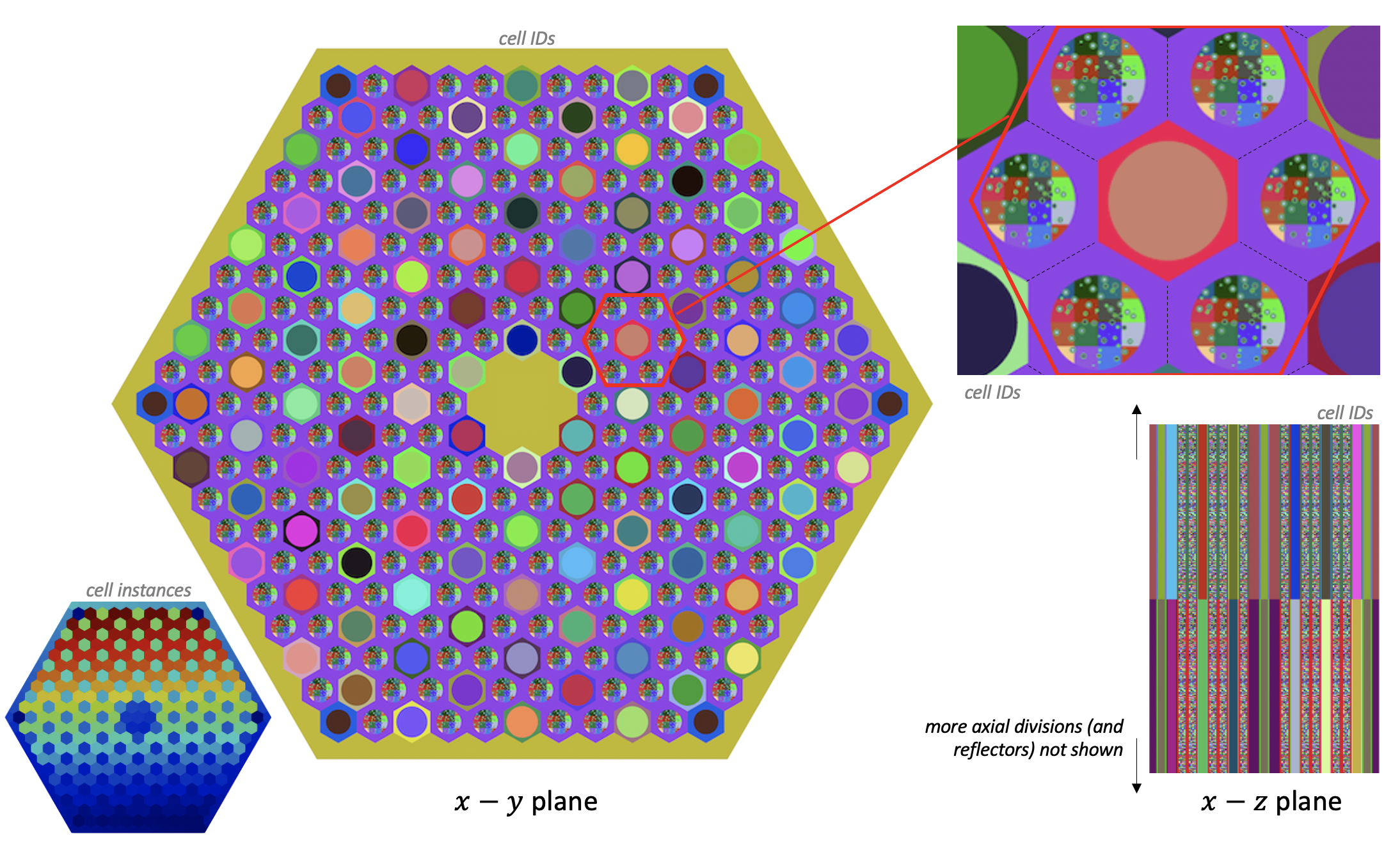
Figure 3: OpenMC model, colored by cell ID or instance

Cardinal applies uniform temperature and density feedback to OpenMC for each unique cell ID $var element = document.getElementById("moose-equation-f492e102-8512-4a5e-974a-cdbce3af9c93");katex.render("+", element, {displayMode:false,throwOnError:false});$ instance combination. For this setup, OpenMC receives on each axial plane a total of 721 temperatures and 108 densities (one density per coolant channel). With references to the colors shown in Figure 3, the 721 cell temperatures correspond to:

$var element = document.getElementById("moose-equation-84266485-3b76-469a-8f8f-527c5254eaf8");katex.render("210\\underbrace{\\text{ fuel compacts}}_{\\substack{\\textup{1 TRISO compact (\\textit{rainbow})}\\\\\\textup{1 matrix region (\\textit{purple})}}}\\ \\ +\\ \\ \\ 108\\underbrace{\\text{ coolant channels}}_{\\substack{\\textup{1 coolant region (\\textit{various})}\\\\\\textup{1 matrix region (\\textit{various})}}}\\ \\ +\\ \\ \\ 6\\underbrace{\\text{ poison compacts}}_{\\substack{\\textup{1 poison region (\\textit{brown})}\\\\\\textup{1 matrix region (\\textit{blue})}}}\\ \\ +\\ \\ \\ 73\\underbrace{\\text{ graphite fillers}}_\\text{1 matrix region (\\textit{mustard})}", element, {displayMode:true,throwOnError:false});$

The solid temperature is provided by the MOOSE heat transfer module, while the fluid temperature and density are provided by THM. Because we will run OpenMC second, the initial fluid temperature is set to the same initial condition that is imposed in the MOOSE solid model. The fluid density is then set using the ideal gas EOS at a fixed pressure of 7.1 MPa given the imposed temperature, i.e. $var element = document.getElementById("moose-equation-cfd647b6-30a8-4c95-97d6-f3f3e48121dd");katex.render("\\rho_f(P,T_f)", element, {displayMode:false,throwOnError:false});$ .

To create the XML files required to run OpenMC, run the script:


python assembly.py

You can also use the XML files checked in to the tutorials/gas_assembly directory; if you use these already-existing files, you will also need to download the geometry.xml file from Box; this file is large due to the saved TRISO geometry information.

THM Model

The Thermal Hydraulics Module (THM) solves for conservation of mass, momentum, and energy with 1-D area averages of the Navier-Stokes equations,

$(2)var element = document.getElementById("moose-equation-78c9ffbb-81fd-4fcd-b992-18399778ac66");katex.render(" \\frac{\\partial}{\\partial t}\\left(A\\rho_f\\right)+\\frac{\\partial}{\\partial x}\\left(A\\rho_fu\\right)=0\\ ,", element, {displayMode:true,throwOnError:false});$

$(3)var element = document.getElementById("moose-equation-03b7b34c-fff0-4f3b-98eb-387f6f5d87f5");katex.render(" \\frac{\\partial}{\\partial t}\\left(A\\rho_fu\\right)+\\frac{\\partial}{\\partial x}\\left(A\\rho_fu^2+AP\\right)=\\tilde{P}\\frac{\\partial A}{\\partial x}-\\frac{f}{2D_h}\\rho_fu|u|A", element, {displayMode:true,throwOnError:false});$

$(4)var element = document.getElementById("moose-equation-bfb94f6f-b77d-47b8-99f2-5739f7b53f8b");katex.render(" \\frac{\\partial}{\\partial t}\\left(A\\rho_f E_f\\right)+\\frac{\\partial}{\\partial x}\\left\\lbrack Au\\left(\\rho_fE_f+P\\right)\\right\\rbrack=H_wa_w\\left(T_\\text{wall}-T_\\text{bulk}\\right)A", element, {displayMode:true,throwOnError:false});$

where $var element = document.getElementById("moose-equation-5641447f-6a89-403a-8d6b-07e737e5dce3");katex.render("x", element, {displayMode:false,throwOnError:false});$ is the coordinate along the flow length, $var element = document.getElementById("moose-equation-f2118bd2-d55b-4716-be6e-1719b8653a8f");katex.render("A", element, {displayMode:false,throwOnError:false});$ is the channel cross-sectional area, $var element = document.getElementById("moose-equation-298424d7-d1e7-4644-bb26-e31d37cb47d9");katex.render("\\rho_f", element, {displayMode:false,throwOnError:false});$ is the fluid density, $var element = document.getElementById("moose-equation-3ab76d10-7587-4fc1-97c2-79d01287b7d4");katex.render("u", element, {displayMode:false,throwOnError:false});$ is the $var element = document.getElementById("moose-equation-ef8e5214-a493-4a19-87ec-3f59ca360442");katex.render("x", element, {displayMode:false,throwOnError:false});$ -component of velocity, $var element = document.getElementById("moose-equation-096f3df9-8881-4979-856d-918c44e6ab0b");katex.render("\\tilde{P}", element, {displayMode:false,throwOnError:false});$ is the average pressure on the curve boundary, $var element = document.getElementById("moose-equation-5b855270-de1c-4499-858a-2729af3f7099");katex.render("E_f", element, {displayMode:false,throwOnError:false});$ is the fluid total energy, $var element = document.getElementById("moose-equation-c48196c9-6878-4f7e-8173-830aa45025ba");katex.render("f", element, {displayMode:false,throwOnError:false});$ is the friction factor, $var element = document.getElementById("moose-equation-84234e47-6cb6-4186-b64e-a37a1030356f");katex.render("H_w", element, {displayMode:false,throwOnError:false});$ is the wall heat transfer coefficient, $var element = document.getElementById("moose-equation-47040489-25e4-4ce5-92e9-7713bf070217");katex.render("a_w", element, {displayMode:false,throwOnError:false});$ is the heat transfer area density, $var element = document.getElementById("moose-equation-56ea5770-1aa0-4db1-9ec3-8a3a0620c675");katex.render("T_\\text{wall}", element, {displayMode:false,throwOnError:false});$ is the wall temperature, and $var element = document.getElementById("moose-equation-12de3e0f-aa66-46e6-a71b-508d35ca4840");katex.render("T_\\text{bulk}", element, {displayMode:false,throwOnError:false});$ is the area average bulk fluid temperature.

In this tutorial, we use 50 elements for each channel. The mesh is constructed automatically within THM. To simplify the specification of material properties, the fluid geometry uses a length unit of meters. The heat flux imposed in the THM elements is obtained by area averaging the heat flux from the heat conduction model in 50 layers along the fluid-solid interface. For the reverse transfer, the wall temperature sent to MOOSE heat conduction is set to a uniform value along the fluid-solid interface according to a nearest-node mapping to the THM elements.

Because THM will run last in the coupled case, initial conditions are only required for pressure, fluid temperature, and velocity, which are set to uniform distributions.

Multiphysics Coupling

A summary of the data transfers between the three applications is shown in Figure 4. The inset describes the 1-D/3-D data transfers with THM.

Figure 4: Summary of data transfers between OpenMC, MOOSE, and THM

Solid Input Files

The solid phase is solved with the MOOSE heat transfer module, and is described in the solid.i input. We define a number of constants at the beginning of the file and set up the mesh from a file.

# copy-pasta from common_input.i
inlet_T = 598.0                          # inlet fluid temperature (K)
buffer_k = 0.5                           # buffer thermal conductivity (W/m/K)
PyC_k = 4.0                              # PyC thermal conductivity (W/m/K)
SiC_k = 13.9                             # SiC thermal conductivity (W/m/K)
kernel_k = 3.5                           # fissil kernel thermal conductivity (W/m/K)
matrix_k = 15.0                          # graphite matrix thermal conductivity (W/m/K)
num_layers_for_plots = 50                # number of layers to average fields over for plotting
triso_pf = 0.15                          # TRISO packing fraction (%)
kernel_radius = 214.85e-6                # fissile kernel outer radius (m)
buffer_radius = 314.85e-6                # buffer outer radius (m)
iPyC_radius = 354.85e-6                  # inner PyC outer radius (m)
SiC_radius = 389.85e-6                   # SiC outer radius (m)
oPyC_radius = 429.85e-6                  # outer PyC outer radius (m)

# compute the volume fraction of each TRISO layer in a TRISO particle
# for use in computing average thermophysical properties
kernel_fraction = ${fparse kernel_radius^3 / oPyC_radius^3}
buffer_fraction = ${fparse (buffer_radius^3 - kernel_radius^3) / oPyC_radius^3}
ipyc_fraction = ${fparse (iPyC_radius^3 - buffer_radius^3) / oPyC_radius^3}
sic_fraction = ${fparse (SiC_radius^3 - iPyC_radius^3) / oPyC_radius^3}
opyc_fraction = ${fparse (oPyC_radius^3 - SiC_radius^3) / oPyC_radius^3}

[Mesh]
  type = FileMesh
  file = solid_mesh_in.e
[]

Next, we define the temperature variable, T, and specify the governing equations and boundary conditions we will apply.

[Variables]
  [T]
    initial_condition = ${inlet_T}
  []
[]

[Kernels]
  [diffusion]
    type = HeatConduction
    variable = T
  []
  [source]
    type = CoupledForce
    variable = T
    v = power
    block = 'compacts'
  []
[]

[BCs]
  [pin_outer]
    type = MatchedValueBC
    variable = T
    v = thm_temp
    boundary = 'fluid_solid_interface'
  []
[]

The MOOSE heat transfer module will receive power from OpenMC in the form of an AuxVariable, so we define a receiver variable for the fission power, as power. The MOOSE heat conduction module will also receive a fluid wall temperature from THM as another AuxVariable which we name thm_temp. Finally, the MOOSE heat transfer module will send the heat flux to THM, so we add a variable named flux that we will use to compute the heat flux using the DiffusionFluxAux auxiliary kernel.

[AuxVariables]
  [thm_temp]
  []
  [flux]
    family = MONOMIAL
    order = CONSTANT
  []
  [power]
    family = MONOMIAL
    order = CONSTANT
  []
[]

[AuxKernels]
  [flux]
    type = DiffusionFluxAux
    diffusion_variable = T
    component = normal
    diffusivity = thermal_conductivity
    variable = flux
    boundary = 'fluid_solid_interface'
  []
[]

We use functions to define the thermal conductivities. The material properties for the TRISO compacts are taken as volume averages of the various constituent materials. We will evaluate the thermal conductivity for the boron carbide as a function of temperature by using t (which usually is interpeted as time) as a variable to represent temperature. This is syntax supported by the HeatConductionMaterials used to apply these functions to the thermal conductivity.

[Functions]
  [k_graphite]
    type = ParsedFunction
    expression = '${matrix_k}'
  []
  [k_TRISO]
    type = ParsedFunction
    expression = '${kernel_fraction} * ${kernel_k} + ${buffer_fraction} * ${buffer_k} + ${fparse ipyc_fraction + opyc_fraction} * ${PyC_k} + ${sic_fraction} * ${SiC_k}'
  []
  [k_compacts]
    type = ParsedFunction
    expression = '${triso_pf} * k_TRISO + ${fparse 1.0 - triso_pf} * k_graphite'
    symbol_names = 'k_TRISO k_graphite'
    symbol_values = 'k_TRISO k_graphite'
  []
  [k_b4c]
    type = ParsedFunction
    expression = '5.096154e-6 * t - 1.952360e-2 * t + 2.558435e1'
  []
[]

[Materials]
  [graphite]
    type = HeatConductionMaterial
    thermal_conductivity_temperature_function = k_graphite
    temp = T
    block = 'graphite'
  []
  [compacts]
    type = HeatConductionMaterial
    thermal_conductivity_temperature_function = k_compacts
    temp = T
    block = 'compacts'
  []
  [poison]
    type = HeatConductionMaterial
    thermal_conductivity_temperature_function = k_b4c
    temp = T
    block = 'poison'
  []
[]

We define a number of postprocessors for querying the solution as well as for normalizing the fission power and heat flux, to be described at greater length in Neutronics Input Files .

[Postprocessors]
  [flux_integral]
    # evaluate the total heat flux for normalization
    type = SideDiffusiveFluxIntegral
    diffusivity = thermal_conductivity
    variable = T
    boundary = 'fluid_solid_interface'
  []
  [max_fuel_T]
    type = ElementExtremeValue
    variable = T
    value_type = max
    block = 'compacts'
  []
  [max_block_T]
    type = ElementExtremeValue
    variable = T
    value_type = max
    block = 'graphite'
  []
  [power]
    # evaluate the total power for normalization
    type = ElementIntegralVariablePostprocessor
    variable = power
    block = 'compacts'
    execute_on = 'transfer'
  []
[]

For visualization purposes only, we add LayeredAverages for the fuel and block temperatures. These will average the temperature in layers oriented in the $var element = document.getElementById("moose-equation-bd321bfc-769d-43de-a841-79dbda0da54d");katex.render("z", element, {displayMode:false,throwOnError:false});$ direction, which we will use for plotting axial temperature distributions. We output the results of these userobjects to CSV using SpatialUserObjectVectorPostprocessors and by setting csv = true in the output.

[UserObjects]
  [average_fuel_axial]
    type = LayeredAverage
    variable = T
    direction = z
    num_layers = ${num_layers_for_plots}
    block = 'compacts'
  []
  [average_block_axial]
    type = LayeredAverage
    variable = T
    direction = z
    num_layers = ${num_layers_for_plots}
    block = 'graphite'
  []
[]

[VectorPostprocessors]
  [fuel_axial_avg]
    type = SpatialUserObjectVectorPostprocessor
    userobject = average_fuel_axial
  []
  [block_axial_avg]
    type = SpatialUserObjectVectorPostprocessor
    userobject = average_block_axial
  []
[]

[Outputs]
  exodus = true
  csv = true
  print_linear_residuals = false
[]

Finally, we specify a Transient executioner. Because there are no time-dependent kernels in this input file, this is equivalent in practice to using a Steady executioner, but allows you to potentially sub-cycle the MOOSE heat conduction solve relative to the OpenMC solve (such as if you wanted to converge the CHT fully inbetween data exchanges with OpenMC).

[Executioner]
  type = Transient
  nl_abs_tol = 1e-5
  nl_rel_tol = 1e-16
  petsc_options_value = 'hypre boomeramg'
  petsc_options_iname = '-pc_type -pc_hypre_type'
[]

Fluid Input Files

The fluid phase is solved with THM, and is described in the thm.i input. This input file is built using syntax specific to THM - we will only briefly cover this syntax, and instead refer users to the THM documentation for more information. First we define a number of constants at the beginning of the file and apply some global settings. We set the initial conditions for pressure, velocity, and temperature and indicate the fluid EOS object using IdealGasFluidProperties.

# copy-pasta from common.i
inlet_T = 598.0                          # inlet fluid temperature (K)
mdot = ${fparse 117.3 / 12 / 108}        # fluid mass flowrate (kg/s)
outlet_P = 7.1e6                         # fluid outlet pressure (Pa)
channel_diameter = 0.016                 # diameter of the coolant channels (m)
height = 6.343                           # height of the assembly (m)

num_layers_for_THM = 50                  # number of elements in the THM model; for the converged case,
                                         # we set this to 150

[GlobalParams]
  initial_p = ${outlet_P}
  initial_T = ${inlet_T}
  initial_vel = ${fparse mdot / outlet_P / 8.3144598 * 4.0e-3 / inlet_T / (pi * channel_diameter * channel_diameter / 4.0)}

  rdg_slope_reconstruction = full
  closures = none
  fp = helium
[]

[Closures]
  [none]
    type = Closures1PhaseNone
  []
[]

[FluidProperties]
  [helium]
    type = IdealGasFluidProperties
    molar_mass = 4e-3
    gamma = 1.668282 # should correspond to  Cp = 5189 J/kg/K
    k = 0.2556
    mu = 3.22639e-5
  []
[]

Next, we define the "components" in the domain. These components essentially consist of the physics equations and boundary conditions solved by THM, but expressed in THM-specific syntax. These components define single-phase flow in a pipe, an inlet mass flowrate boundary condition, an outlet pressure boundary condition, and heat transfer to the pipe wall.

[Components]
  [channel]
    type = FlowChannel1Phase
    position = '0 0 ${height}'
    orientation = '0 0 -1'

    A = '${fparse pi * channel_diameter * channel_diameter / 4}'
    D_h = ${channel_diameter}
    length = ${height}
    n_elems = ${num_layers_for_THM}
  []

  [inlet]
    type = InletMassFlowRateTemperature1Phase
    input = 'channel:in'
    m_dot = ${mdot}
    T = ${inlet_T}
  []

  [outlet]
    type = Outlet1Phase
    input = 'channel:out'
    p = ${outlet_P}
  []

  [ht_ext]
    type = HeatTransferFromExternalAppHeatFlux1Phase
    flow_channel = channel
    P_hf = '${fparse channel_diameter * pi}'
  []
[]

Associated with these components are a number of closures, defined as materials. We set up the Churchill correlation for the friction factor and the Dittus-Boelter correlation for the convective heat transfer coefficient. Additional materials are created to represent dimensionless numbers and other auxiliary terms, such as the wall temperature. As can be seen here, the Material system is not always used to represent quantities traditionally thought of as "material properties."

[Materials]
  # wall friction closure
  [f_mat]
    type = ADWallFrictionChurchillMaterial
    block = channel
    D_h = D_h
    f_D = f_D
    vel = vel
    rho = rho
    mu = mu
  []

  # Wall heat transfer closure (all important is in Nu_mat)
  [Re_mat]
    type = ADReynoldsNumberMaterial
    block = channel
    Re = Re
    D_h = D_h
    mu = mu
    vel = vel
    rho = rho
  []
  [Pr_mat]
    type = ADPrandtlNumberMaterial
    block = channel
    cp = cp
    mu = mu
    k = k
  []
  [Nu_mat]
    type = ADParsedMaterial
    block = channel
    # Dittus-Boelter
    expression = '0.022 * pow(Re, 0.8) * pow(Pr, 0.4)'
    property_name = 'Nu'
    material_property_names = 'Re Pr'
  []
  [Hw_mat]
    type = ADConvectiveHeatTransferCoefficientMaterial
    block = channel
    D_h = D_h
    Nu = Nu
    k = k
  []
  [T_wall]
    type = ADTemperatureWall3EqnMaterial
    Hw = Hw
    T = T
    q_wall = q_wall
  []
[]

THM computes the wall temperature to apply a boundary condition in the MOOSE heat transfer module. To convert the T_wall material into an auxiliary variable, we use the ADMaterialRealAux.

[AuxVariables]
  [T_wall]
    family = MONOMIAL
    order = CONSTANT
  []
[]

[AuxKernels]
  [Tw_aux]
    type = ADMaterialRealAux
    block = channel
    variable = T_wall
    property = T_wall
  []
[]

Finally, we set the preconditioner, a Transient executioner, and set an Exodus output. The steady_state_detection and steady_state_tolerance parameters will automatically terminate the THM solution once the relative change in the solution is less than $var element = document.getElementById("moose-equation-462666a8-20c8-4168-942b-23e56a492c30");katex.render("10^{-8}", element, {displayMode:false,throwOnError:false});$ .

[Preconditioning]
  [pc]
    type = SMP
    full = true
  []
[]

[Executioner]
  type = Transient
  dt = 0.1
  start_time = 0

  steady_state_detection = true
  steady_state_tolerance = 1e-08

  nl_rel_tol = 1e-5
  nl_abs_tol = 1e-6

  petsc_options_iname = '-pc_type'
  petsc_options_value = 'lu'

  solve_type = NEWTON
  line_search = basic
[]

[Outputs]
  exodus = true
  print_linear_residuals = false

  [console]
    type = Console
    outlier_variable_norms = false
  []
[]

As you may notice, this THM input file only models a single coolant flow channel. We will leverage a feature in MOOSE that allows a single application to be repeated multiple times throughout a main application without having to merge input files or perform other transformations. We will run OpenMC as the main application; the syntax needed to achieve this setup is covered next.

Neutronics Input Files

The neutronics physics is solved with OpenMC over the entire domain. The OpenMC wrapping is described in the openmc.i file. We begin by defining a number of constants and by setting up the mesh mirror on which OpenMC will receive temperature and density from the coupled applications, and on which OpenMC will write the fission heat source. Because the coupled MOOSE applications use length units of meters, the mesh mirror must also be in units of meters in order to obtain correct data transfers. For simplicity, we use the same solid mesh as used by the solid heat conduction solution, but this is not required. For the fluid region, we use MOOSE mesh generators to construct a mesh for a single coolant channel, and then repeat it for the 108 coolant channels.

num_layers_for_THM = 50      # number of elements in the THM model; for the converged
                             # case, we set this to 150

[Mesh]
  # mesh mirror for the solid regions
  [solid]
    type = FileMeshGenerator
    file = solid_mesh_in.e
  []

  # create a mesh for a single coolant channel; because we will receive uniform
  # temperatures and densities from THM on each x-y plane, we can use a very coarse
  # mesh in the radial direction
  [coolant_face]
    type = AnnularMeshGenerator
    nr = 1
    nt = 8
    rmin = 0.0
    rmax = ${fparse channel_diameter / 2.0}
  []
  [extrude]
    type = AdvancedExtruderGenerator
    input = coolant_face
    num_layers = ${num_layers_for_THM}
    direction = '0 0 1'
    heights = '${height}'
    top_boundary = '300' # inlet
    bottom_boundary = '400' # outlet
  []
  [rename]
    type = RenameBlockGenerator
    input = extrude
    old_block = '1'
    new_block = '101'
  []

  # repeat the coolant channels and then combine together to get a combined mesh mirror
  [repeat]
    type = CombinerGenerator
    inputs = rename
    positions_file = coolant_channel_positions.txt
  []
  [add]
    type = CombinerGenerator
    inputs = 'solid repeat'
  []
[]

Before progressing further, we first need to describe the multiapp structure connecting OpenMC, MOOSE heat conduction, and THM. We set the main application to OpenMC, and will have both MOOSE heat conduction and THM as "sibling" sub-applications.

note

At the time of writing, the MOOSE framework does not support "sibling" multiapp transfers, meaning that the data to be communicated between MOOSE heat conduction and THM (the heat flux and wall temperature data transfers in Figure 4) must go "up a level" to their common main application. This has since been relaxed.

Therefore, we will see in the OpenMC input file information related to data transfers between MOOSE heat conduction and THM. The auxiliary variables defined for the OpenMC model are shown below.

[AuxVariables]
  [material_id]
    family = MONOMIAL
    order = CONSTANT
  []
  [cell_temperature]
    family = MONOMIAL
    order = CONSTANT
  []
  [cell_density]
    family = MONOMIAL
    order = CONSTANT
  []
  [thm_temp_wall]
    block = '101'
  []
  [flux]
  []

  # just for postprocessing purposes
  [thm_pressure]
    block = '101'
  []
  [thm_velocity]
    block = '101'
  []
  [z]
    family = MONOMIAL
    order = CONSTANT
    block = 'compacts'
  []
[]

[AuxKernels]
  [material_id]
    type = CellMaterialIDAux
    variable = material_id
  []
  [cell_temperature]
    type = CellTemperatureAux
    variable = cell_temperature
  []
  [cell_density]
    type = CellDensityAux
    variable = cell_density
  []
  [density]
    type = FluidDensityAux
    variable = density
    p = ${outlet_P}
    T = thm_temp
    fp = helium
    execute_on = 'timestep_begin linear'
  []
  [z]
    type = ParsedAux
    variable = z
    use_xyzt = true
    expression = 'z'
  []
[]

For visualization purposes, we use a CellTemperatureAux to view the temperature set in each OpenMC cell and a CellDensityAux to view the density set in each fluid OpenMC cell. To understand how the OpenMC model maps to the [Mesh], we also include CellMaterialIDAux. Cardinal will also automatically output a variable named cell_id (CellIDAux) and a variable named cell_instance ( CellInstanceAux) to show the spatial mapping. Next, we add a receiver flux variable that will hold the heat flux received from MOOSE (and sent to THM) and another receiver variable thm_temp_wall that will hold the wall temperature received from THM (and sent to MOOSE).

Finally, to reduce the number of transfers from THM, we will receive fluid temperature from THM, but re-compute the density locally in the OpenMC wrapping using a FluidDensityAux with the same EOS as used in the THM input files.

[FluidProperties]
  [helium]
    type = IdealGasFluidProperties
    molar_mass = 4e-3
    gamma = 1.668282 # should correspond to  Cp = 5189 J/kg/K
    k = 0.2556
    mu = 3.22639e-5
  []
[]

Next, we set initial conditions for the fluid wall temperature, the fluid bulk temperature, and the heat source. We set these initial conditions in the OpenMC wrapper because the very first time that the transfers to the MOOSE heat conduction module and to THM occur, these initial conditions will be passed.

[ICs]
  [fluid_temp_wall]
    type = FunctionIC
    variable = thm_temp_wall
    function = temp_ic
  []
  [fluid_temp]
    type = FunctionIC
    variable = thm_temp
    function = temp_ic
  []
  [heat_source]
    type = ConstantIC
    variable = heat_source
    block = 'compacts'
    value = ${fparse power / (n_bundles * n_fuel_compacts_per_block) / (pi * compact_diameter * compact_diameter / 4.0 * height)}
  []
[]

[Functions]
  [temp_ic]
    type = ParsedFunction
    expression = '${inlet_T} + (${height} - z) / ${height} * ${power} / ${mdot} / ${fluid_Cp}'
  []
[]

The [Problem] and [Tallies] blocks are then used to specify settings for the OpenMC wrapping. We define the total power for normalization, indicate that blocks 1, 2, and 4 are solid (graphite, compacts, and poison) while block 101 is fluid. We add a CellTally to block 2, the fuel compacts. Because OpenMC solves in units of centimeters, we specify a scaling of 100, i.e. a multiplicative factor to apply to the [Mesh] to get into OpenMC's centimeter units.

[Problem]
  type = OpenMCCellAverageProblem

  identical_cell_fills = '2'

  power = '${fparse power / n_bundles}'
  scaling = 100.0
  cell_level = 1

  relaxation = constant
  relaxation_factor = 0.5

  # to get a faster-running tutorial, we use only 1000 particles per batch; converged
  # results are instead obtained by increasing this parameter to 10000. We also use fewer
  # batches to speed things up; the converged results were obtained with 500 inactive batches
  # and 2000 active batches
  particles = 1000
  inactive_batches = 200
  batches = 1000

  # we will read temperature from THM (for the fluid) and MOOSE (for the solid)
  # into variables we name as 'solid_temp' and 'thm_temp'. This syntax will automatically
  # create those variabes for us
  temperature_variables = 'solid_temp; thm_temp'
  temperature_blocks = '1 2 4;      101'
  density_blocks = '101'

  [Tallies]
    [heat_source]
      type = CellTally
      blocks = '2'
      name = heat_source
      check_equal_mapped_tally_volumes = true
      output = 'unrelaxed_tally_std_dev'
    []
  []
[]

Other features we use include an output of the fission tally standard deviation in units of W/m $var element = document.getElementById("moose-equation-ca51ce83-5929-4157-b1d8-d611b506b99b");katex.render("^3", element, {displayMode:false,throwOnError:false});$ to the [Mesh] by setting output = 'unrelaxed_tally_std_dev'. This is used to obtain uncertainty estimates of the heat source distribution from OpenMC in the same units as the heat source. We also leverage a helper utility in CellTally by setting check_equal_mapped_tally_volumes = true. This parameter will throw an error if the tallied OpenMC cells map to different volumes in the MOOSE domain. Because we know a priori that the equal-volume OpenMC tally cells should all map to equal volumes, this will help ensure that the volumes used for heat source normalization are also all equal. For further discussion of this setting and a pictorial description of the possible effect of non-equal mapped vlumes, please see the OpenMCCellAverageProblem documentation.

We also set identical_cell_fills to the set of subdomains for which OpenMC's cells have identical fills. This is an optimization that greatly reduces the initialization time for large TRISO problems. During setup of an OpenMC wrapping, we need to cache all the cells contained within the TRISO compacts so that we know all the contained cells to set the temperatures for. This process can be quite time-consuming if the search needs to be repeated for every single TRISO compact cell (210 compacts times 50 axial layers = 10,500 contained cell searches). The identical_cell_fills option is used to indicate whether your problem can leverage a speedup that applies to models where every lattice/universe-filled tally cell has exactly the same filling lattice/universe. In other words, we set up our problem to use the same TRISO universe in each layer of each fuel compact. This means that the cells filling each TRISO compact can be deduced by following a pattern based on the first two fuel compacts, letting us omit 10,498 of the contained cell searches.

note

When first using this optimization for a new problem, we recommend setting check_identical_cell_fills = true so that you can do an exact comparison against the "rigorous" approach to be sure that your problem setup has the necessary prerequisites to use this feature. After you verify that no errors are thrown during setup, set check_identical_cell_fills to false (the default) to use this initialization speedup feature.

Because the blocks in the OpenMC mesh mirror receive temperatures from different applications, we use the temperature_variables and temperature_blocks parameters of OpenMCCellAverageProblem to automatically create separate variables for OpenMC to read temperature from in different parts of the domain. The temperature_blocks and temperature_variables parameters allow you to customize exactly the variable names from which to read temperature.

Finally, we apply a constant relaxation model to the heat source. A constant relaxation will compute the heat source in iteration $var element = document.getElementById("moose-equation-738e350b-73c9-46d7-b7d4-8b58f17356c6");katex.render("i+1", element, {displayMode:false,throwOnError:false});$ as an average of the heat source from iteration $var element = document.getElementById("moose-equation-18accee8-349b-45df-bfd1-4485e35f4a16");katex.render("i", element, {displayMode:false,throwOnError:false});$ and the most-recently-computed heat source, indicated here as a generic operator $var element = document.getElementById("moose-equation-0dae402f-d960-4e2e-8bd8-29eea6bacafb");katex.render("\\Phi", element, {displayMode:false,throwOnError:false});$ which represents the Monte Carlo solve:

$(5)var element = document.getElementById("moose-equation-03b33a6b-7927-4d03-8e56-d4eb5f034c09");katex.render(" q^{i+1}=\\left(1-\\alpha\\right)q^i+\\alpha\\Phi", element, {displayMode:true,throwOnError:false});$

In Eq. (5), $var element = document.getElementById("moose-equation-0dce5784-88de-406b-8111-67bbaa929d0b");katex.render("\\alpha", element, {displayMode:false,throwOnError:false});$ is the relaxation factor, which we set here to 0.5. In other words, the heat source in iteration $var element = document.getElementById("moose-equation-234f8f95-e48e-469a-a993-954f7737619e");katex.render("i+1", element, {displayMode:false,throwOnError:false});$ is an average of the most recent Monte Carlo solution and the previous iterate. This is necessary to accelerate the fixed point iterations and achieve convergence in a reasonable time - otherwise oscillations can occur in the coupled physics.

We run OpenMC as the main application, so we next need to define MultiApps to run the solid heat conduction model and the THM fluid model as the sub-applications. We also require a number of transfers both for 1) sending necessary coupling data between the three applications and 2) visualizing the combined THM output. To couple OpenMC to MOOSE heat conduction, we use four transfers:

MultiAppShapeEvaluationTransfer to transfer:
- power from OpenMC to MOOSE (with conservation of total power)
MultiAppGeometricInterpolationTransfer to transfer:
- solid temperature from MOOSE to OpenMC
- wall temperature from OpenMC (which doesn't directly compute the wall temperature, but instead receives it from THM through a separate transfer) to MOOSE
MultiAppGeneralFieldNearestLocationTransfer to transfer and conserve heat flux from MOOSE to OpenMC (which isn't used directly in OpenMC, but instead gets sent later to THM through a separate transfer)

To couple OpenMC to THM, we require three transfers:

MultiAppGeneralFieldUserObjectTransfer to send the layer-averaged wall heat flux from OpenMC (which computes the layered-average heat flux from the heat flux received from MOOSE heat conduction) to THM
MultiAppGeneralFieldNearestLocationTransfer to transfer:
- fluid wall temperature from THM to OpenMC (which isn't used directly in OpenMC, but instead gets sent to MOOSE heat conduction in a separate transfer)
- fluid bulk temperature from THM to OpenMC

For visualization purposes, we also send the pressure and velocity computed by THM to the OpenMC mesh mirror.

[MultiApps]
  [bison]
    type = TransientMultiApp
    input_files = 'solid.i'
    execute_on = timestep_begin
  []
  [thm]
    type = FullSolveMultiApp
    input_files = 'thm.i'
    execute_on = timestep_end
    max_procs_per_app = 1
    bounding_box_padding = '0.1 0.1 0'
    positions_file = coolant_channel_positions.txt
    output_in_position = true
  []
[]

[Transfers]
  [solid_temp_to_openmc]
    type = MultiAppGeometricInterpolationTransfer
    source_variable = T
    variable = solid_temp
    from_multi_app = bison
  []
  [heat_flux_to_openmc]
    type = MultiAppGeneralFieldNearestLocationTransfer
    source_variable = flux
    variable = flux
    from_multi_app = bison
    from_boundaries = 'fluid_solid_interface'
    to_boundaries = 'fluid_solid_interface'
    from_postprocessors_to_be_preserved = flux_integral
    to_postprocessors_to_be_preserved = flux_integral
  []
  [source_to_bison]
    type = MultiAppGeneralFieldShapeEvaluationTransfer
    source_variable = heat_source
    variable = power
    to_multi_app = bison
    from_postprocessors_to_be_preserved = heat_source
    to_postprocessors_to_be_preserved = power
  []
  [thm_temp_to_bison]
    type = MultiAppGeometricInterpolationTransfer
    source_variable = thm_temp_wall
    variable = thm_temp
    to_multi_app = bison
  []

  [q_wall_to_thm]
    type = MultiAppGeneralFieldUserObjectTransfer
    variable = q_wall
    to_multi_app = thm
    source_user_object = q_wall_avg
  []
  [T_wall_from_thm]
    type = MultiAppGeneralFieldNearestLocationTransfer
    source_variable = T_wall
    from_multi_app = thm
    variable = thm_temp_wall
    to_boundaries = 'fluid_solid_interface'
  []
  [T_bulk_from_thm]
    type = MultiAppGeneralFieldNearestLocationTransfer
    source_variable = T
    from_multi_app = thm
    variable = thm_temp
  []

  # just for postprocessing purposes
  [pressure_from_thm]
    type = MultiAppGeneralFieldNearestLocationTransfer
    source_variable = p
    from_multi_app = thm
    variable = thm_pressure
  []
  [velocity_from_thm]
    type = MultiAppGeneralFieldNearestLocationTransfer
    source_variable = vel_z
    from_multi_app = thm
    variable = thm_velocity
  []
[]

To compute the layer-averaged heat flux on the surface of each coolant channel (which is used as a boundary condition in THM), we use a NearestPointLayeredSideAverage user object, where by providing the center points of each of the coolant channels, we can get a unique heat flux along each channel wall. We also add several LayeredAverage user objects in order to compute radially-averaged power, temperatures, pressures, and velocities that we will use later in making axial plots of the solution. We can automatically output these user objects into CSV format by translating the user objects into SpatialUserObjectVectorPostprocessors. A number of postprocessors are included related to the Monte Carlo solution, as well as inlet pressure and pressure drop. See the next section for further description.

[UserObjects]
  [q_wall_avg]
    type = NearestPointLayeredSideAverage
    boundary = 'fluid_solid_interface'
    variable = flux

    # Note: make this to match the num_elems in the channel
    direction = z
    num_layers = ${num_layers_for_THM}
    points_file = coolant_channel_positions.txt

    direction_min = 0.0
    direction_max = ${height}
  []
  [average_power_axial]
    type = LayeredAverage
    variable = heat_source
    direction = z
    num_layers = ${num_layers_for_plots}
    block = 'compacts'
  []
  [average_fluid_axial]
    type = LayeredAverage
    variable = thm_temp
    direction = z
    num_layers = ${num_layers_for_plots}
    block = '101'
  []
  [average_pressure]
    type = LayeredAverage
    variable = thm_pressure
    direction = z
    num_layers = ${num_layers_for_plots}
    block = '101'
  []
  [average_axial_velocity]
    type = LayeredAverage
    variable = thm_velocity
    direction = z
    num_layers = ${num_layers_for_plots}
    block = '101'
  []
[]

[VectorPostprocessors]
  [power_avg]
    type = SpatialUserObjectVectorPostprocessor
    userobject = average_power_axial
  []
  [fluid_avg]
    type = SpatialUserObjectVectorPostprocessor
    userobject = average_fluid_axial
  []
  [pressure_avg]
    type = SpatialUserObjectVectorPostprocessor
    userobject = average_pressure
  []
  [velocity_avg]
    type = SpatialUserObjectVectorPostprocessor
    userobject = average_axial_velocity
  []
[]

[Postprocessors]
  [flux_integral]
    type = SideIntegralVariablePostprocessor
    variable = flux
    boundary = 'fluid_solid_interface'
    execute_on = 'transfer linear'
  []
  [heat_source]
    type = ElementIntegralVariablePostprocessor
    variable = heat_source
    execute_on = 'transfer initial timestep_end'
  []
  [max_tally_rel_err]
    type = TallyRelativeError
    value_type = max
  []
  [k]
    type = KEigenvalue
  []
  [k_std_dev]
    type = KStandardDeviation
  []
  [min_power]
    type = ElementExtremeValue
    variable = heat_source
    value_type = min
    block = 'compacts'
  []
  [max_power]
    type = ElementExtremeValue
    variable = heat_source
    value_type = max
    block = 'compacts'
  []
  [z_max_power]
    type = ElementExtremeValue
    proxy_variable = heat_source
    variable = z
    block = 'compacts'
  []
  [max_Tf]
    type = ElementExtremeValue
    variable = thm_temp
    block = '101'
  []
  [P_in]
    type = SideAverageValue
    variable = thm_pressure
    boundary = '300'
  []
  [pressure_drop]
    type = LinearCombinationPostprocessor
    pp_names = 'P_in'
    pp_coefs = '1.0'
    b = '${fparse -outlet_P}'
  []
[]

Finally, we use a Transient executioner and specify Exodus and CSV output formats. Note that the time step size is inconsequential in this case, but instead represents the Picard iteration. We will run for 10 "time steps," which represent fixed point iterations.

[Executioner]
  type = Transient
  num_steps = 10
[]

[Outputs]
  exodus = true
  csv = true
  hide = 'P_in flux_integral z'
[]

Execution and Postprocessing

To run the coupled calculation,


mpiexec -np 4 cardinal-opt -i common_input.i openmc.i --n-threads=2

This will run with 4 MPI processes and 2 OpenMP threads per rank. This tutorial uses quite large meshes due to the 6 meter height of the domain - if you wish to run this tutorial with fewer computational resources, you can reduce the height and the various mesh parameters (number of extruded layers and elements in the THM domain) and then recreate the OpenMC model and meshes. Recall that all results shown in this section correspond to the same input files but with 300 extrusion layers in the solid, 150 THM elements per channel, 2000 particles per batch, 500 inactive batches, and 2000 active batches - to get a faster-running tutorial, we reduced all of these parameters to coarser values.

When the simulation has completed, you will have created a number of different output files:

openmc_out.e, an Exodus file with the OpenMC solution and the data that was ultimately transferred in/out of OpenMC
openmc_out_bison0.e, an Exodus file with the solid solution
openmc_out_thm<n>.e, Exodus files with each of the <n> THM solutions
openmc_out.csv, a CSV file with the results of the postprocessors in the OpenMC wrapping input file for each time step
openmc_out_bison0.csv, a CSV file with the results of the postprocessors in the solid heat conduction input file for each time step
openmc_out_bison0_block_axial_avg_<n>.csv, a CSV file with the layer-averaged block temperature at time step <n>
openmc_out_bison0_flux_axial_avg_<n>.csv, a CSV file with the layer-averaged fluid-solid interface heat flux at time step <n>
openmc_out_bison0_fuel_axial_avg_<n>.csv, a CSV file with the layer-averaged compact temperature at time step <n>
openmc_out_fluid_avg_<n>.csv, a CSV file with the layer-averaged fluid bulk temperature at time step <n>
openmc_out_power_avg_<n>.csv, a CSV file with the layer-averaged heat source at time step <n>
openmc_out_pressure_avg_<n>.csv, a CSV file with the layer-averaged pressure at time step <n>
openmc_out_velocity_avg_<n>.csv, a CSV file with the layer-average axial fluid velocity at time step <n>

Coupled convergence is defined at the point when 1) the $var element = document.getElementById("moose-equation-ab5e8660-0117-473a-bc9a-b8abe622a1c0");katex.render("k", element, {displayMode:false,throwOnError:false});$ eigenvalue is within the uncertainty band of the previous iteration and 2) there is less than 2 K absolute change in maximum fuel, block, and fluid temperatures. Convergence is obtained in 6 fixed point iterations. Figure 5 shows the maximum fuel, compact, and fluid temperatures, along with the $var element = document.getElementById("moose-equation-8423a5ca-e506-4018-91bd-4faff2936a36");katex.render("k", element, {displayMode:false,throwOnError:false});$ eigenvalue, as a function of iteration number for all 10 iterations run. For each iteration, we first run MOOSE heat conduction (which we indicate as iterations A1, A2, and so on), followed by OpenMC (which we indicate as iterations B1, B2, and so on), and finally THM (which we indicate as iterations C1, C2, and so on). In other words, in iteration $var element = document.getElementById("moose-equation-a0b98448-dc86-4c4d-814f-7cbf129c9b01");katex.render("i", element, {displayMode:false,throwOnError:false});$ :

Iteration A $var element = document.getElementById("moose-equation-598176ac-9c3d-4d51-b4dd-9c2cdcda3b3b");katex.render("i", element, {displayMode:false,throwOnError:false});$ represents a MOOSE heat conduction solve using the power and fluid-solid wall temperature from iteration $var element = document.getElementById("moose-equation-ebdb09ed-bc03-4275-894d-e65a3212e47c");katex.render("i-1", element, {displayMode:false,throwOnError:false});$
Iteration B $var element = document.getElementById("moose-equation-fb51f7a3-9a67-48f2-a958-7292e8485af1");katex.render("i", element, {displayMode:false,throwOnError:false});$ represents an OpenMC solve using the solid temperature from iteration $var element = document.getElementById("moose-equation-adae0e82-518b-497f-bdc7-240faba9012b");katex.render("i", element, {displayMode:false,throwOnError:false});$ and the fluid temperature and density from iteration $var element = document.getElementById("moose-equation-61532a54-491d-4757-8f0a-19750d41c300");katex.render("i-1", element, {displayMode:false,throwOnError:false});$
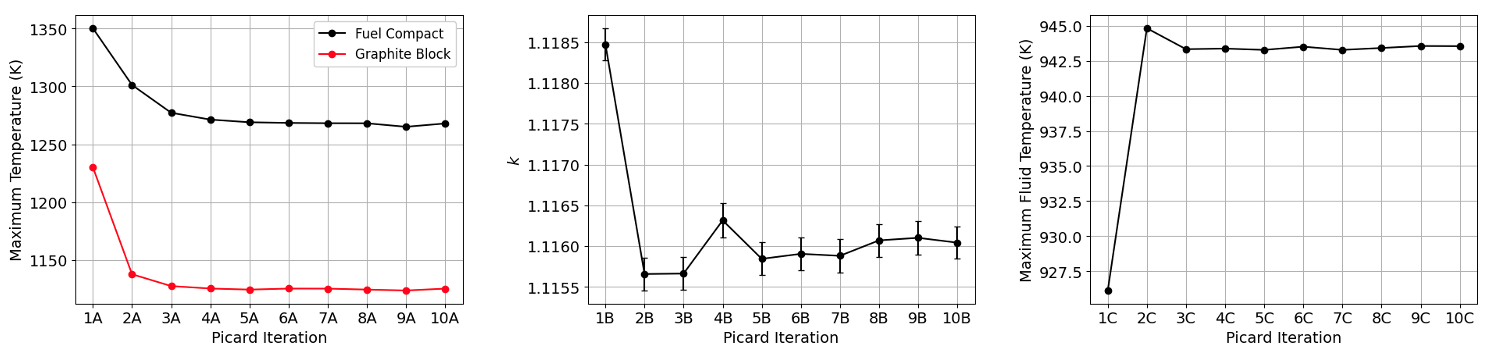
Iteration C $var element = document.getElementById("moose-equation-60e182e7-98d8-4f8c-83ae-d54622b89db9");katex.render("i", element, {displayMode:false,throwOnError:false});$ represents a THM solve using the fluid-solid wall heat flux from iteration $var element = document.getElementById("moose-equation-f88e1187-0bbe-4ae4-b472-650f0be8bf7a");katex.render("i", element, {displayMode:false,throwOnError:false});$

Figure 5: Convergence in various metrics as a function of iteration number

Figure 6 shows the radially-averaged power from OpenMC as a function of iteration number. There is essentially no change in the axial distribution beyond 6 fixed point iterations, which further confirms that we have obtained a converged solution. The remainder of the depicted results correpond to iteration 6.

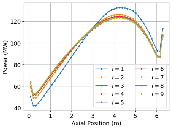
Figure 6: Radially-average fission power distribution as a function of iteration number $var element = document.getElementById("moose-equation-1f16c018-05dc-47e4-9085-646172597d50");katex.render("i", element, {displayMode:false,throwOnError:false});$

Figure 7 shows the fission power distribution computed by OpenMC. The inset shows the power distribution on an $var element = document.getElementById("moose-equation-755ef8c9-5950-41cc-81c8-0744f6d3481b");katex.render("x-y", element, {displayMode:false,throwOnError:false});$ plane 2.15 meters from the inlet, where the maximum power occurs. Slight azimuthal asymmetries exist due to the finite tally uncertainty. Neutrons reflecting back into the fuel region from the axial reflectors cause local power peaking at the ends of the assembly, while the negative fuel temperature coefficient causes the power distribution to shift towards the reactor inlet where temperatures are lower. The six poison compacts in the corners result in local power depression such that the highest compact powers occur near the center of the assembly.

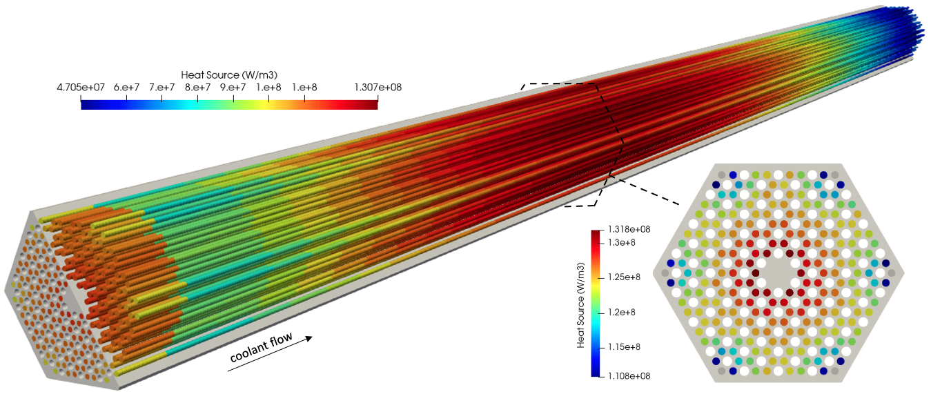
Figure 7: Fission power predicted by OpenMC; note the use of a separate color scale for the inset.

Figure 8 shows the solid temperature (left) computed by MOOSE and the cell temperature imposed in OpenMC (right). The bottom row shows the temperature on an $var element = document.getElementById("moose-equation-4a95459a-e832-4235-ba51-1535cfc4d348");katex.render("x-y", element, {displayMode:false,throwOnError:false});$ plane 2.15 meters from the inlet. The insulated boundary conditions, combined with a lower "density" of coolant channels near the lateral faces, result in higher compact temperatures near the assembly peripheries, except in the vicinity of the poison pins where the increased absorption reduces the local power densities. Each OpenMC cell is set to the volume-average temperature from the mesh mirror elements whose centroids mapped to each cell; a similar procedure is used to set cell temperatures and densities for the fluid cells.

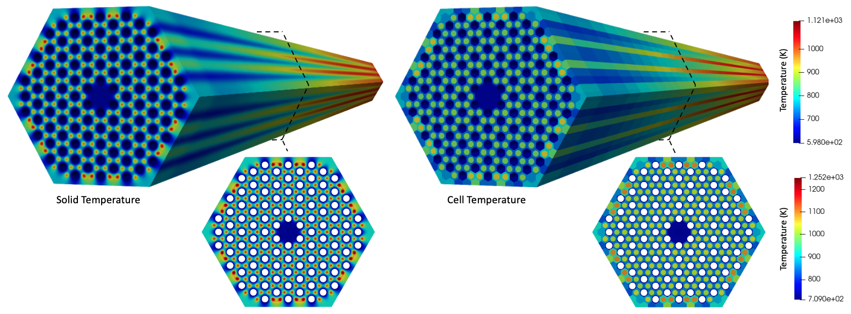
Figure 8: Solid temperature predicted by MOOSE (left) and volume-average temperature imposed in OpenMC (right). Note the use of a separate color scale for the insets.

Figure 9 shows the solid temperature computed by MOOSE on several $var element = document.getElementById("moose-equation-7f5bee0a-6a09-4e6a-ac02-8ea57be0cfdb");katex.render("x-y", element, {displayMode:false,throwOnError:false});$ planes with the fluid temperature computed by THM shown as tubes. An inset shows the fluid temperature on the outlet plane. The absence of compacts in the center region results in the lowest fluid temperatures in this region, while the highest fluid temperatures are observed for channels surrounded by 6 compacts that are sufficiently close to the periphery to be affected by the lateral insulated boundary conditions.

Figure 9: Fluid temperature predicted by THM (tubes and inset) and solid temperature predicted by MOOSE (five slices). Note the use of three separate color scales.

Finally, Figure 10 shows the radially-averaged fission distribution and fluid, compact, and graphite temperatures (left); and velocity and pressure (right) as a function of axial position. The negative temperature feedback results in a top-peaked power distribution. The fuel temperature peaks near the mid-plane due to the combined effects of the relatively high power density and the continually-increasing fluid temperature with distance from the inlet. The pressure gradient is nearly constant with axial position. Due to mass conservation, the heating of the fluid results in the velocity increasing with distance from the inlet.

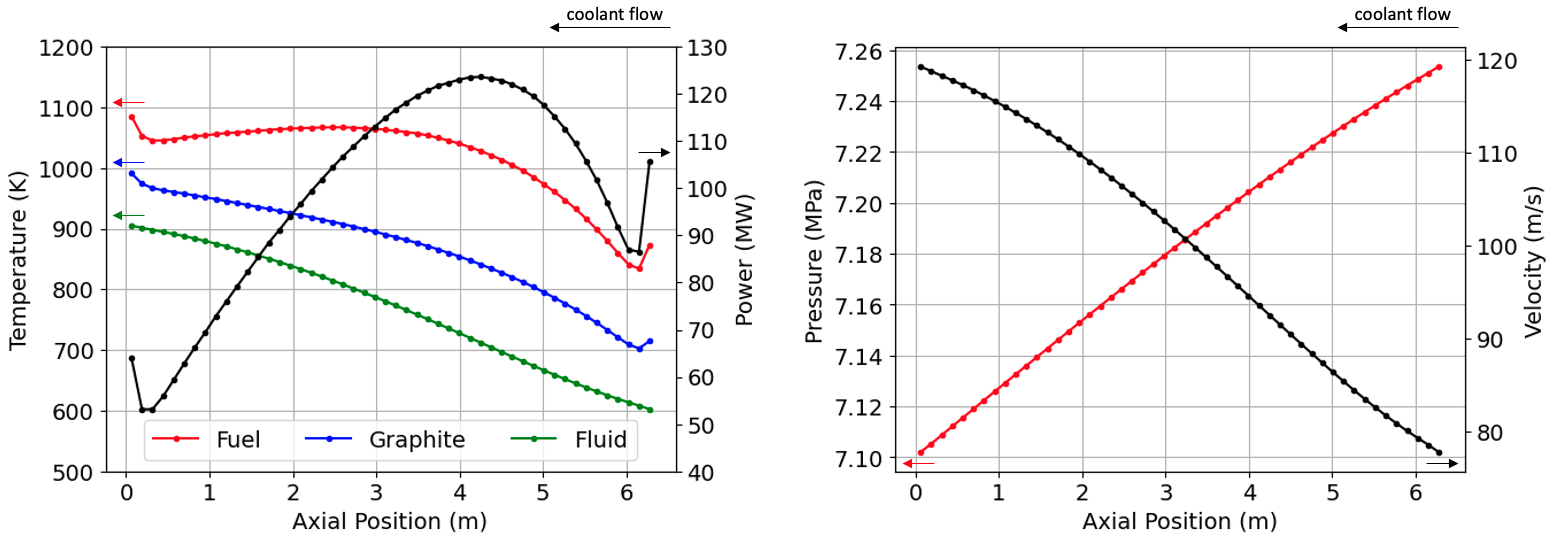
Figure 10: Radially-averaged temperatures, power, pressure, and velocity as a function of position.

References

INL. High-Temperature Gas-Cooled Test Reactor Point Design. Technical Report INL/EXT-16-38296, Idaho National Laboratory, 2016. URL: https://tinyurl.com/v9a4hym5.

@TechReport{sterbentz,
    author = "INL",
    title = "{High-Temperature Gas-Cooled Test Reactor Point Design}",
    institution = "Idaho National Laboratory",
    year = "2016",
    number = "INL/EXT-16-38296",
    url = "https://tinyurl.com/v9a4hym5"
}

A.J. Novak, D. Andrs, P. Shriwise, D. Shaver, P.K. Romano, E. Merzari, and P. Keutelian. Coupled Monte Carlo and Thermal-Hydraulics Modeling of a Prismatic Gas Reactor Fuel Assembly Using Cardinal. In Proceedings of Physor. 2021.

@InProceedings{novak_2021c,
    author = "Novak, A.J. and Andrs, D. and Shriwise, P. and Shaver, D. and Romano, P.K. and Merzari, E. and Keutelian, P.",
    title = "{Coupled {Monte} {Carlo} and Thermal-Hydraulics Modeling of a Prismatic Gas Reactor Fuel Assembly Using {Cardinal}}",
    booktitle = "{Proceedings of Physor}",
    year = "2021"
}

E. Shemon, K. Mo, Y. Miao, Y. Jung, S. Richards, A. Oaks, and S. Kumar. MOOSE Framework Enhancements for Meshing Reactor Geometries. In Proceedings of Physor. 2021.

@InProceedings{shemon_2021,
    author = "Shemon, E. and Mo, K. and Miao, Y. and Jung, Y. and Richards, S. and Oaks, A. and Kumar, S.",
    title = "{{MOOSE} Framework Enhancements for Meshing Reactor Geometries}",
    booktitle = "{Proceedings of Physor}",
    year = "2021"
}

(tutorials/gas_assembly/solid_mesh.i)

n_layers = 100    # number of axial extrusion layers; for the converged case,
                  # we set this to 300 to get a finer mesh

[GlobalParams]
  quad_center_elements = true
[]

[Mesh]
  [fuel_pin]
    type = PolygonConcentricCircleMeshGenerator
    num_sides = 6
    polygon_size = ${fparse fuel_to_coolant_distance / 2.0}
    ring_radii = '${fparse 0.8 * compact_diameter / 2.0} ${fparse compact_diameter / 2.0}'
    ring_intervals = '1 1'
    num_sectors_per_side = '4 4 4 4 4 4'
    ring_block_ids = '2 2'
    ring_block_names = 'compacts compacts'
    background_block_ids = '1'
    background_block_names = 'graphite'
    background_intervals = 2
  []
  [coolant_pin]
    type = PolygonConcentricCircleMeshGenerator
    num_sides = 6
    polygon_size = ${fparse fuel_to_coolant_distance / 2.0}
    ring_radii = '${fparse channel_diameter / 2.0}'
    ring_intervals = '2'
    num_sectors_per_side = '4 4 4 4 4 4'
    ring_block_ids = '101 101'
    ring_block_names = 'coolant coolant'
    background_block_ids = '1'
    background_block_names = 'graphite'
    interface_boundary_id_shift = 100
    create_inward_interface_boundaries = true
    background_intervals = 2
  []
  [poison_pin]
    type = PolygonConcentricCircleMeshGenerator
    num_sides = 6
    polygon_size = ${fparse fuel_to_coolant_distance / 2.0}
    ring_radii = '${fparse compact_diameter / 2.0}'
    ring_intervals = '2'
    num_sectors_per_side = '4 4 4 4 4 4'
    ring_block_ids = '4 4'
    ring_block_names = 'poison poison'
    background_block_ids = '1'
    background_block_names = 'graphite'
    background_intervals = 2
  []
  [graphite_pin]
    type = PolygonConcentricCircleMeshGenerator
    num_sides = 6
    polygon_size = ${fparse fuel_to_coolant_distance / 2.0}
    ring_radii = '${fparse compact_diameter / 2.0}'
    ring_intervals = '2'
    num_sectors_per_side = '4 4 4 4 4 4'
    ring_block_ids = '1 1'
    ring_block_names = 'graphite graphite'
    background_block_ids = '1'
    background_block_names = 'graphite'
  []
  [bundle]
    type = PatternedHexMeshGenerator
    inputs = 'fuel_pin coolant_pin poison_pin graphite_pin'
    hexagon_size = ${fparse bundle_flat_to_flat / 2.0 + bundle_gap_width / 2.0}
    pattern = '2 0 1 0 0 1 0 0 1 0 2;
              0 1 0 0 1 0 0 1 0 0 1 0;
             1 0 0 1 0 0 1 0 0 1 0 0 1;
            0 0 1 0 0 1 0 0 1 0 0 1 0 0;
           0 1 0 0 1 0 0 1 0 0 1 0 0 1 0;
          1 0 0 1 0 0 1 0 0 1 0 0 1 0 0 1;
         0 0 1 0 0 1 0 0 1 0 0 1 0 0 1 0 0;
        0 1 0 0 1 0 0 1 0 0 1 0 0 1 0 0 1 0;
       1 0 0 1 0 0 1 0 0 1 0 0 1 0 0 1 0 0 1;
      0 0 1 0 0 1 0 0 1 3 3 1 0 0 1 0 0 1 0 0;
     2 1 0 0 1 0 0 1 0 3 3 3 0 1 0 0 1 0 0 1 2;
      0 0 1 0 0 1 0 0 1 3 3 1 0 0 1 0 0 1 0 0;
       1 0 0 1 0 0 1 0 0 1 0 0 1 0 0 1 0 0 1;
        0 1 0 0 1 0 0 1 0 0 1 0 0 1 0 0 1 0;
         0 0 1 0 0 1 0 0 1 0 0 1 0 0 1 0 0;
          1 0 0 1 0 0 1 0 0 1 0 0 1 0 0 1;
           0 1 0 0 1 0 0 1 0 0 1 0 0 1 0;
            0 0 1 0 0 1 0 0 1 0 0 1 0 0;
             1 0 0 1 0 0 1 0 0 1 0 0 1;
              0 1 0 0 1 0 0 1 0 0 1 0;
               2 0 1 0 0 1 0 0 1 0 2'
    rotate_angle = 0

    background_block_id = '1'
  []
  [extrude]
    type = AdvancedExtruderGenerator
    input = bundle
    heights = ${height}
    num_layers = ${n_layers}
    direction = '0 0 1'
  []
  [delete_coolant]
    type = BlockDeletionGenerator
    input = extrude
    block = '101'
  []
  [rename_coolant_sideset]
    type = RenameBoundaryGenerator
    input = delete_coolant
    old_boundary = 102
    new_boundary = 'fluid_solid_interface'
  []

  construct_side_list_from_node_list = true
[]

# The following content is adding postprocessor(s) to check sideset areas.
# The reactor module is unfortunately quite brittle in its assignment of sideset
# IDs, so we want to be extra sure that any changes to sideset numbering are detected
# in our test suite.
[Problem]
  type = FEProblem
  solve = false
[]

[Postprocessors]
  [area_walls]
    type = AreaPostprocessor
    boundary = 'fluid_solid_interface'
  []
[]

[Executioner]
  type = Steady
[]

[Outputs]
  csv = true
  exodus = true
[]

(tutorials/gas_assembly/assembly.py)

#!/bin/env python
#********************************************************************/
#*                  SOFTWARE COPYRIGHT NOTIFICATION                 */
#*                             Cardinal                             */
#*                                                                  */
#*                  (c) 2021 UChicago Argonne, LLC                  */
#*                        ALL RIGHTS RESERVED                       */
#*                                                                  */
#*                 Prepared by UChicago Argonne, LLC                */
#*               Under Contract No. DE-AC02-06CH11357               */
#*                With the U. S. Department of Energy               */
#*                                                                  */
#*             Prepared by Battelle Energy Alliance, LLC            */
#*               Under Contract No. DE-AC07-05ID14517               */
#*                With the U. S. Department of Energy               */
#*                                                                  */
#*                 See LICENSE for full restrictions                */
#********************************************************************/

from argparse import ArgumentParser
import math
import numpy as np
import matplotlib.pyplot as plt

import openmc
import sys
import os

# Get common input parameters shared by other physics
script_dir = os.path.dirname(__file__)
sys.path.append(script_dir)
import common_input as specs

def coolant_temp(t_in, t_out, l, z):
    """
    Computes the coolant temperature based on an expected cosine power distribution
    for a specified temperature rise. The total core temperature rise is governed
    by energy conservation as dT = Q / m / Cp, where dT is the total core temperature
    rise, Q is the total core power, m is the mass flowrate, and Cp is the fluid
    isobaric specific heat. If you neglect axial heat conduction and assume steady
    state, then the temperature rise in a layer of fluid i can be related to the
    ratio of the power in that layer to the total power,
    dT_i / dT = Q_i / Q. We assume here a sinusoidal power distribution to get
    a reasonable estimate of an initial coolant temperature distribution.

    Parameters
    ----------

    t_in : float
        Inlet temperature of the channel
    t_out : float
        Outlet temperature of the channel
    l : float
        Length of the channel
    z : float or 1-D numpy.array
        Axial position where the temperature will be computed

    Returns
    -------
        float or 1-D numpy array of float depending on z
    """
    dT = t_out - t_in
    Q = 2 * l / math.pi
    Qi = (l - l * np.cos(math.pi * z / l)) / math.pi

    t = t_in + Qi / Q * dT

    return t

def coolant_density(t):
  """
  Computes the helium density (kg/m3) from temperature assuming a fixed operating pressure.

  Parameters
  ----------

  t : float
    Fluid temperature

  Returns
  _______
    float or 1-D numpy array of float depending on t
  """

  p_in_bar = specs.outlet_P * 1.0e-5
  return 48.14 * p_in_bar / (t + 0.4446 * p_in_bar / math.pow(t, 0.2))

# -------------- Unit Conversions: OpenMC requires cm -----------
m = 100.0

# estimate the outlet temperature using bulk energy conservation for steady state
coolant_outlet_temp = specs.power / specs.mdot / specs.fluid_Cp + specs.inlet_T

# geometry parameters
coolant_channel_diam = specs.channel_diameter * m
reactor_bottom = 0.0
reactor_height = specs.height * m
reactor_top = reactor_bottom + reactor_height
bundle_pitch = specs.bundle_flat_to_flat * m + specs.bundle_gap_width * m
cell_pitch = specs.fuel_to_coolant_distance * m
fuel_channel_diam = specs.compact_diameter * m
top_reflector_height = specs.top_reflector_thickness * m
bottom_reflector_height = specs.bottom_reflector_thickness * m

def assembly(n_ax_zones, n_inactive, n_active, add_entropy_mesh=False):
    axial_section_height = reactor_height / n_ax_zones

    # superimposed search lattice
    triso_lattice_shape = (4, 4, int(axial_section_height / 0.05))

    model = openmc.model.Model()

    enrichment = 0.155        # U-235 enrichment (weight percent)
    enrichment_234 = 2e-3     # U-234 enrichment (weight percent)
    kernel_density = 10820    # fissile kernel density (kg/m3)
    buffer_density = 1050     # buffer density (kg/m3)
    PyC_density = 1900        # PyC density (kg/m3)
    SiC_density = 3203        # SiC density (kg/m3)
    matrix_density = 1700     # graphite matrix density (kg/m3)

    # ----- uranium oxycarbide fuel ----- #
    m_fuel = openmc.Material(name='fuel')
    mass_234 = openmc.data.atomic_mass('U234')
    mass_235 = openmc.data.atomic_mass('U235')
    mass_238 = openmc.data.atomic_mass('U238')

    n_234 = enrichment_234 / mass_234
    n_235 = enrichment / mass_235
    n_238 = (1.0 - enrichment - enrichment_234) / mass_238
    total_n = n_234 + n_235 + n_238

    m_fuel.add_nuclide('U234', n_234 / total_n)
    m_fuel.add_nuclide('U235', n_235 / total_n)
    m_fuel.add_nuclide('U238', n_238 / total_n)
    m_fuel.add_element('C'   , 1.50)
    m_fuel.add_element('O'   , 0.50)
    m_fuel.set_density('kg/m3', kernel_density)

    # ----- graphite buffer ----- #
    m_graphite_c_buffer = openmc.Material(name='buffer')
    m_graphite_c_buffer.add_element('C', 1.0)
    m_graphite_c_buffer.add_s_alpha_beta('c_Graphite')
    m_graphite_c_buffer.set_density('kg/m3', buffer_density)

    # ----- pyrolitic carbon ----- #
    m_graphite_pyc = openmc.Material(name='pyc')
    m_graphite_pyc.add_element('C', 1.0)
    m_graphite_pyc.add_s_alpha_beta('c_Graphite')
    m_graphite_pyc.set_density('kg/m3', PyC_density)

    # ----- silicon carbide ----- #
    m_sic = openmc.Material(name='sic')
    m_sic.add_element('C' , 1.0)
    m_sic.add_element('Si', 1.0)
    m_sic.set_density('kg/m3', SiC_density)

    # ----- matrix graphite ----- #
    m_graphite_matrix = openmc.Material(name='graphite moderator')
    m_graphite_matrix.add_element('C', 1.0)
    m_graphite_matrix.add_s_alpha_beta('c_Graphite')
    m_graphite_matrix.set_density('kg/m3', matrix_density)

    # ----- helium coolant ----- #
    m_coolant = openmc.Material(name='Helium coolant')
    m_coolant.add_element('He', 1.0, 'ao')
    # we don't set density here because we'll set it as a function of temperature

    m_b4c = openmc.Material(name='B4C')
    enrichment_10 = specs.B10_enrichment
    mass_10 = openmc.data.atomic_mass('B10')
    mass_11 = openmc.data.atomic_mass('B11')

    # number of atoms in one gram of boron mixture
    n_10 = enrichment_10 / mass_10
    n_11 = (1.0 - enrichment_10) / mass_11
    total_n = n_10 + n_11
    grams_10 = n_10 / total_n
    grams_11 = n_11 / total_n

    # now, figure out how much carbon needs to be in the poison to get
    # an overall specified B10 weight percent
    total_b10_weight_percent = specs.total_B10_wt_percent
    total_mass = grams_10 / total_b10_weight_percent
    carbon_mass = total_mass - grams_10 - grams_11

    m_b4c.add_nuclide('B10', grams_10 / total_mass, 'wo')
    m_b4c.add_nuclide('B11', grams_11 / total_mass, 'wo')
    m_b4c.add_element('C', carbon_mass / total_mass, 'wo')
    m_b4c.set_density('kg/m3', specs.B4C_density)

    # reflector is 40 percent helium by volume (arbitrary assumption), with helium
    # at the inlet conditions
    rho = coolant_density(specs.inlet_T) # kg/m3
    reflector_porosity = 0.40
    n_helium = reflector_porosity * rho / 4.002602
    n_carbon = (1.0 - reflector_porosity) * matrix_density / 12.0107
    combined_density = rho * reflector_porosity + matrix_density * (1.0 - reflector_porosity)
    m_reflector = openmc.Material(name='reflector')
    m_reflector.add_element('He', n_helium / (n_helium + n_carbon))
    m_reflector.add_element('C', n_carbon / (n_helium + n_carbon))
    m_reflector.set_density('kg/m3', combined_density)

    # TRISO particle
    radius_pyc_outer   = specs.oPyC_radius * m

    s_fuel             = openmc.Sphere(r=specs.kernel_radius*m)
    s_c_buffer         = openmc.Sphere(r=specs.buffer_radius*m)
    s_pyc_inner        = openmc.Sphere(r=specs.iPyC_radius*m)
    s_sic              = openmc.Sphere(r=specs.SiC_radius*m)
    s_pyc_outer        = openmc.Sphere(r=radius_pyc_outer)
    c_triso_fuel       = openmc.Cell(name='c_triso_fuel'     , fill=m_fuel,              region=-s_fuel)
    c_triso_c_buffer   = openmc.Cell(name='c_triso_c_buffer' , fill=m_graphite_c_buffer, region=+s_fuel      & -s_c_buffer)
    c_triso_pyc_inner  = openmc.Cell(name='c_triso_pyc_inner', fill=m_graphite_pyc,      region=+s_c_buffer  & -s_pyc_inner)
    c_triso_sic        = openmc.Cell(name='c_triso_sic'      , fill=m_sic,               region=+s_pyc_inner & -s_sic)
    c_triso_pyc_outer  = openmc.Cell(name='c_triso_pyc_outer', fill=m_graphite_pyc,      region=+s_sic       & -s_pyc_outer)
    c_triso_matrix     = openmc.Cell(name='c_triso_matrix'   , fill=m_graphite_matrix,   region=+s_pyc_outer)
    u_triso            = openmc.Universe(cells=[c_triso_fuel, c_triso_c_buffer, c_triso_pyc_inner, c_triso_sic, c_triso_pyc_outer, c_triso_matrix])

    # Channel surfaces
    fuel_cyl = openmc.ZCylinder(r=0.5 * fuel_channel_diam)
    coolant_cyl = openmc.ZCylinder(r=0.5 * coolant_channel_diam)
    poison_cyl = openmc.ZCylinder(r=0.5 * fuel_channel_diam)
    graphite_cyl = openmc.ZCylinder(r=0.5 * fuel_channel_diam)

    # create a TRISO lattice for one axial section (to be used in the rest of the axial zones)
    # center the TRISO region on the origin so it fills lattice cells appropriately
    min_z = openmc.ZPlane(z0=-0.5 * axial_section_height)
    max_z = openmc.ZPlane(z0=0.5 * axial_section_height)

    # region in which TRISOs are generated
    r_triso = -fuel_cyl & +min_z & -max_z

    rand_spheres = openmc.model.pack_spheres(radius=radius_pyc_outer, region=r_triso, pf=specs.triso_pf, seed=1.0)
    random_trisos = [openmc.model.TRISO(radius_pyc_outer, u_triso, i) for i in rand_spheres]

    llc, urc = r_triso.bounding_box
    pitch = (urc - llc) / triso_lattice_shape

    # insert TRISOs into a lattice to accelerate point location queries
    triso_lattice = openmc.model.create_triso_lattice(random_trisos, llc, pitch, triso_lattice_shape, m_graphite_matrix)

    axial_coords = np.linspace(reactor_bottom, reactor_top, n_ax_zones + 1)
    lattice_univs = []
    bundle_univs = []

    m_colors = {}

    for z_min, z_max in zip(axial_coords[0:-1], axial_coords[1:]):
        # use the middle of the axial section to compute the temperature and density
        ax_pos = 0.5 * (z_min + z_max)
        T = coolant_temp(specs.inlet_T, coolant_outlet_temp, reactor_height, ax_pos)

        # create solid cells, which don't require us to clone materials in order to set temperatures
        fuel_ch_cell = openmc.Cell(region=-fuel_cyl, fill=triso_lattice)
        fuel_ch_cell.temperature = T

        fuel_ch_matrix_cell = openmc.Cell(region=+fuel_cyl, fill=m_graphite_matrix)
        fuel_ch_matrix_cell.temperature = T

        poison_cell = openmc.Cell(region=-poison_cyl, fill=m_b4c)
        poison_cell.temperature = T

        poison_matrix_cell = openmc.Cell(region=+poison_cyl, fill=m_graphite_matrix)
        poison_matrix_cell.temperature = T

        graphite_cell = openmc.Cell(fill=m_graphite_matrix)
        graphite_cell.temperature = T

        coolant_matrix_cell = openmc.Cell(region=+coolant_cyl, fill=m_graphite_matrix)
        coolant_matrix_cell.temperature = T

        # create fluid cells, which require us to clone the material in order to be able to
        # set unique densities
        coolant_cell = openmc.Cell(region=-coolant_cyl, fill=m_coolant)
        coolant_cell.fill = [m_coolant.clone() for i in range(specs.n_coolant_channels_per_block)]

        for mat in range(len(coolant_cell.fill)):
          m_colors[coolant_cell.fill[mat]] = 'red'

        # Define a universe for each type of solid-only pin (fuel, poison, and graphite)
        f = openmc.Universe(cells=[fuel_ch_cell, fuel_ch_matrix_cell])
        p = openmc.Universe(cells=[poison_cell, poison_matrix_cell])
        c = openmc.Universe(cells=[coolant_cell, coolant_matrix_cell])
        g = openmc.Universe(cells=[graphite_cell])

        d = [f] * 2

        ring2 = ([f] + [c]) * 6
        ring3 = ([c] + d) * 6
        ring4 = (d + [c] + [f]) * 6
        ring5 = ([f] + [c] + d + [c]) * 6
        ring6 = ([c] + d + [c] + d) * 6
        ring7 = (d + [c] + d + [c] + [f]) * 6
        ring8 = ([f] + [c] + d + [c] + d + [c]) * 6
        ring9 = ([c] + d + [c] + d + [c] + d) * 6
        ring10 = ([p] + [f] + [c] + d + [c] + d + [c] + [f]) * 6
        ring11 = [g] * 66

        # inner two rings where there aren't any fuel/compact/poison pins
        ring1 = [g] * 6
        ring0 = [g]

        lattice_univs.append([ring11, ring10, ring9, ring8, ring7, ring6, ring5, ring4, ring3, ring2, ring1, ring0])

    # create a hexagonal lattice used in each axial zone to represent the cell
    hex_lattice = openmc.HexLattice(name="Bundle cell lattice")
    hex_lattice.orientation = 'x'
    hex_lattice.center = (0.0, 0.0, 0.5 * (reactor_bottom + reactor_top))
    hex_lattice.pitch = (cell_pitch, axial_section_height)
    hex_lattice.universes = lattice_univs

    hexagon_volume = reactor_height * math.sqrt(3) / 2.0 * bundle_pitch**2
    coolant_channel_volume = math.pi * coolant_channel_diam**2 / 4.0 * reactor_height

    graphite_outer_cell = openmc.Cell(fill=m_graphite_matrix)
    graphite_outer_cell.temperature = T
    inf_graphite_univ = openmc.Universe(cells=[graphite_outer_cell])
    hex_lattice.outer = inf_graphite_univ

    # create additional axial regions
    axial_planes = [openmc.ZPlane(z0=coord) for coord in axial_coords]

    # axial planes
    min_z = axial_planes[0]
    max_z = axial_planes[-1]

    # fill the unit cell with the hex lattice
    hex_prism = openmc.model.HexagonalPrism(bundle_pitch / math.sqrt(3.0), 'x', boundary_type='periodic')
    outer_cell = openmc.Cell(region=-hex_prism & +min_z & -max_z, fill=hex_lattice)

    # add the top and bottom reflector
    top_refl_z = reactor_height + top_reflector_height
    top_refl = openmc.ZPlane(z0=top_refl_z, boundary_type='vacuum')
    bottom_refl_z = -bottom_reflector_height
    bottom_refl = openmc.ZPlane(z0=bottom_refl_z, boundary_type='vacuum')

    top_refl_cell = openmc.Cell(region=-hex_prism & +max_z & -top_refl, fill=m_reflector)
    bottom_refl_cell = openmc.Cell(region=-hex_prism & -min_z & +bottom_refl, fill=m_reflector)
    top_refl_cell.temperature = specs.inlet_T
    bottom_refl_cell.temperature = coolant_outlet_temp

    model.geometry = openmc.Geometry([outer_cell, top_refl_cell, bottom_refl_cell])

    ### Settings ###
    settings = openmc.Settings()

    settings.particles = 10000
    settings.inactive = n_inactive
    settings.batches = settings.inactive + n_active
    settings.temperature['method'] = 'interpolation'
    settings.temperature['range'] = (294.0, 1500.0)

    l = bundle_pitch / math.sqrt(3.0)
    lower_left = (-l, -l, reactor_bottom)
    upper_right = (l, l, reactor_top)
    source_dist = openmc.stats.Box(lower_left, upper_right, only_fissionable=True)
    source = openmc.IndependentSource(space=source_dist)
    settings.source = source

    if (add_entropy_mesh):
        entropy_mesh = openmc.RegularMesh()
        entropy_mesh.lower_left = lower_left
        entropy_mesh.upper_right = upper_right
        entropy_mesh.dimension = (6, 6, 20)
        settings.entropy_mesh = entropy_mesh

    vol_calc = openmc.VolumeCalculation([outer_cell],
                                        100_000_000, lower_left, upper_right)
    settings.volume_calculations = [vol_calc]

    model.settings = settings

    m_colors[m_fuel] = 'palegreen'
    m_colors[m_graphite_c_buffer] = 'sandybrown'
    m_colors[m_graphite_pyc] = 'orange'
    m_colors[m_sic] = 'yellow'
    m_colors[m_graphite_matrix] = 'darkblue'
    m_colors[m_b4c] = 'lightskyblue'

    bundle_p_rounded = int(bundle_pitch)

    plot1          = openmc.Plot()
    plot1.filename = 'plot1'
    plot1.width    = (2 * bundle_pitch, 2 * axial_section_height)
    plot1.basis    = 'xz'
    plot1.origin   = (0.0, 0.0, reactor_height / 2.0)
    plot1.pixels   = (100 * 2 * bundle_p_rounded, int(100 * 3 * axial_section_height))
    plot1.color_by = 'cell'

    plot2          = openmc.Plot()
    plot2.filename = 'plot2'
    plot2.width    = (1.5 * bundle_pitch, 1.5 * bundle_pitch)
    plot2.basis    = 'xy'
    plot2.origin   = (0.0, 0.0, axial_section_height / 4.0)
    plot2.pixels   = (500 * bundle_p_rounded, 500 * bundle_p_rounded)
    plot2.color_by = 'material'
    plot2.colors   = m_colors

    plot3          = openmc.Plot()
    plot3.filename = 'plot3'
    plot3.width    = plot2.width
    plot3.basis    = plot2.basis
    plot3.origin   = plot2.origin
    plot3.pixels   = plot2.pixels
    plot3.color_by = 'cell'

    model.plots = openmc.Plots([plot1, plot2, plot3])

    return model


def main():

    ap = ArgumentParser()
    ap.add_argument('-n', dest='n_axial', type=int, default=50,
                    help='Number of axial cell divisions')
    ap.add_argument('-s', '--entropy', action='store_true',
                    help='Whether to add a Shannon entropy mesh')
    ap.add_argument('-i', dest='n_inactive', type=int, default=500,
                    help='Number of inactive cycles')
    ap.add_argument('-a', dest='n_active', type=int, default=2000,
                    help='Number of active cycles')

    args = ap.parse_args()

    model = assembly(args.n_axial, args.n_inactive, args.n_active, args.entropy)
    model.export_to_xml()

if __name__ == "__main__":
    main()

(tutorials/gas_assembly/solid.i)

# copy-pasta from common_input.i
inlet_T = 598.0                          # inlet fluid temperature (K)
buffer_k = 0.5                           # buffer thermal conductivity (W/m/K)
PyC_k = 4.0                              # PyC thermal conductivity (W/m/K)
SiC_k = 13.9                             # SiC thermal conductivity (W/m/K)
kernel_k = 3.5                           # fissil kernel thermal conductivity (W/m/K)
matrix_k = 15.0                          # graphite matrix thermal conductivity (W/m/K)
num_layers_for_plots = 50                # number of layers to average fields over for plotting
triso_pf = 0.15                          # TRISO packing fraction (%)
kernel_radius = 214.85e-6                # fissile kernel outer radius (m)
buffer_radius = 314.85e-6                # buffer outer radius (m)
iPyC_radius = 354.85e-6                  # inner PyC outer radius (m)
SiC_radius = 389.85e-6                   # SiC outer radius (m)
oPyC_radius = 429.85e-6                  # outer PyC outer radius (m)

# compute the volume fraction of each TRISO layer in a TRISO particle
# for use in computing average thermophysical properties
kernel_fraction = ${fparse kernel_radius^3 / oPyC_radius^3}
buffer_fraction = ${fparse (buffer_radius^3 - kernel_radius^3) / oPyC_radius^3}
ipyc_fraction = ${fparse (iPyC_radius^3 - buffer_radius^3) / oPyC_radius^3}
sic_fraction = ${fparse (SiC_radius^3 - iPyC_radius^3) / oPyC_radius^3}
opyc_fraction = ${fparse (oPyC_radius^3 - SiC_radius^3) / oPyC_radius^3}

[Mesh]
  type = FileMesh
  file = solid_mesh_in.e
[]

[Variables]
  [T]
    initial_condition = ${inlet_T}
  []
[]

[Kernels]
  [diffusion]
    type = HeatConduction
    variable = T
  []
  [source]
    type = CoupledForce
    variable = T
    v = power
    block = 'compacts'
  []
[]

[BCs]
  [pin_outer]
    type = MatchedValueBC
    variable = T
    v = thm_temp
    boundary = 'fluid_solid_interface'
  []
[]

[Functions]
  [k_graphite]
    type = ParsedFunction
    expression = '${matrix_k}'
  []
  [k_TRISO]
    type = ParsedFunction
    expression = '${kernel_fraction} * ${kernel_k} + ${buffer_fraction} * ${buffer_k} + ${fparse ipyc_fraction + opyc_fraction} * ${PyC_k} + ${sic_fraction} * ${SiC_k}'
  []
  [k_compacts]
    type = ParsedFunction
    expression = '${triso_pf} * k_TRISO + ${fparse 1.0 - triso_pf} * k_graphite'
    symbol_names = 'k_TRISO k_graphite'
    symbol_values = 'k_TRISO k_graphite'
  []
  [k_b4c]
    type = ParsedFunction
    expression = '5.096154e-6 * t - 1.952360e-2 * t + 2.558435e1'
  []
[]

[Materials]
  [graphite]
    type = HeatConductionMaterial
    thermal_conductivity_temperature_function = k_graphite
    temp = T
    block = 'graphite'
  []
  [compacts]
    type = HeatConductionMaterial
    thermal_conductivity_temperature_function = k_compacts
    temp = T
    block = 'compacts'
  []
  [poison]
    type = HeatConductionMaterial
    thermal_conductivity_temperature_function = k_b4c
    temp = T
    block = 'poison'
  []
[]

[Postprocessors]
  [flux_integral] # evaluate the total heat flux for normalization
    type = SideDiffusiveFluxIntegral
    diffusivity = thermal_conductivity
    variable = T
    boundary = 'fluid_solid_interface'
  []
  [max_fuel_T]
    type = ElementExtremeValue
    variable = T
    value_type = max
    block = 'compacts'
  []
  [max_block_T]
    type = ElementExtremeValue
    variable = T
    value_type = max
    block = 'graphite'
  []
  [power] # evaluate the total power for normalization
    type = ElementIntegralVariablePostprocessor
    variable = power
    block = 'compacts'
    execute_on = 'transfer'
  []
[]

[AuxVariables]
  [thm_temp]
  []
  [flux]
    family = MONOMIAL
    order = CONSTANT
  []
  [power]
    family = MONOMIAL
    order = CONSTANT
  []
[]

[AuxKernels]
  [flux]
    type = DiffusionFluxAux
    diffusion_variable = T
    component = normal
    diffusivity = thermal_conductivity
    variable = flux
    boundary = 'fluid_solid_interface'
  []
[]

[Executioner]
  type = Transient
  nl_abs_tol = 1e-5
  nl_rel_tol = 1e-16
  petsc_options_value = 'hypre boomeramg'
  petsc_options_iname = '-pc_type -pc_hypre_type'
[]

[UserObjects]
  [average_fuel_axial]
    type = LayeredAverage
    variable = T
    direction = z
    num_layers = ${num_layers_for_plots}
    block = 'compacts'
  []
  [average_block_axial]
    type = LayeredAverage
    variable = T
    direction = z
    num_layers = ${num_layers_for_plots}
    block = 'graphite'
  []
[]

[VectorPostprocessors]
  [fuel_axial_avg]
    type = SpatialUserObjectVectorPostprocessor
    userobject = average_fuel_axial
  []
  [block_axial_avg]
    type = SpatialUserObjectVectorPostprocessor
    userobject = average_block_axial
  []
[]

[Outputs]
  exodus = true
  csv = true
  print_linear_residuals = false
[]

(tutorials/gas_assembly/solid.i)

# copy-pasta from common_input.i
inlet_T = 598.0                          # inlet fluid temperature (K)
buffer_k = 0.5                           # buffer thermal conductivity (W/m/K)
PyC_k = 4.0                              # PyC thermal conductivity (W/m/K)
SiC_k = 13.9                             # SiC thermal conductivity (W/m/K)
kernel_k = 3.5                           # fissil kernel thermal conductivity (W/m/K)
matrix_k = 15.0                          # graphite matrix thermal conductivity (W/m/K)
num_layers_for_plots = 50                # number of layers to average fields over for plotting
triso_pf = 0.15                          # TRISO packing fraction (%)
kernel_radius = 214.85e-6                # fissile kernel outer radius (m)
buffer_radius = 314.85e-6                # buffer outer radius (m)
iPyC_radius = 354.85e-6                  # inner PyC outer radius (m)
SiC_radius = 389.85e-6                   # SiC outer radius (m)
oPyC_radius = 429.85e-6                  # outer PyC outer radius (m)

# compute the volume fraction of each TRISO layer in a TRISO particle
# for use in computing average thermophysical properties
kernel_fraction = ${fparse kernel_radius^3 / oPyC_radius^3}
buffer_fraction = ${fparse (buffer_radius^3 - kernel_radius^3) / oPyC_radius^3}
ipyc_fraction = ${fparse (iPyC_radius^3 - buffer_radius^3) / oPyC_radius^3}
sic_fraction = ${fparse (SiC_radius^3 - iPyC_radius^3) / oPyC_radius^3}
opyc_fraction = ${fparse (oPyC_radius^3 - SiC_radius^3) / oPyC_radius^3}

[Mesh]
  type = FileMesh
  file = solid_mesh_in.e
[]

[Variables]
  [T]
    initial_condition = ${inlet_T}
  []
[]

[Kernels]
  [diffusion]
    type = HeatConduction
    variable = T
  []
  [source]
    type = CoupledForce
    variable = T
    v = power
    block = 'compacts'
  []
[]

[BCs]
  [pin_outer]
    type = MatchedValueBC
    variable = T
    v = thm_temp
    boundary = 'fluid_solid_interface'
  []
[]

[Functions]
  [k_graphite]
    type = ParsedFunction
    expression = '${matrix_k}'
  []
  [k_TRISO]
    type = ParsedFunction
    expression = '${kernel_fraction} * ${kernel_k} + ${buffer_fraction} * ${buffer_k} + ${fparse ipyc_fraction + opyc_fraction} * ${PyC_k} + ${sic_fraction} * ${SiC_k}'
  []
  [k_compacts]
    type = ParsedFunction
    expression = '${triso_pf} * k_TRISO + ${fparse 1.0 - triso_pf} * k_graphite'
    symbol_names = 'k_TRISO k_graphite'
    symbol_values = 'k_TRISO k_graphite'
  []
  [k_b4c]
    type = ParsedFunction
    expression = '5.096154e-6 * t - 1.952360e-2 * t + 2.558435e1'
  []
[]

[Materials]
  [graphite]
    type = HeatConductionMaterial
    thermal_conductivity_temperature_function = k_graphite
    temp = T
    block = 'graphite'
  []
  [compacts]
    type = HeatConductionMaterial
    thermal_conductivity_temperature_function = k_compacts
    temp = T
    block = 'compacts'
  []
  [poison]
    type = HeatConductionMaterial
    thermal_conductivity_temperature_function = k_b4c
    temp = T
    block = 'poison'
  []
[]

[Postprocessors]
  [flux_integral] # evaluate the total heat flux for normalization
    type = SideDiffusiveFluxIntegral
    diffusivity = thermal_conductivity
    variable = T
    boundary = 'fluid_solid_interface'
  []
  [max_fuel_T]
    type = ElementExtremeValue
    variable = T
    value_type = max
    block = 'compacts'
  []
  [max_block_T]
    type = ElementExtremeValue
    variable = T
    value_type = max
    block = 'graphite'
  []
  [power] # evaluate the total power for normalization
    type = ElementIntegralVariablePostprocessor
    variable = power
    block = 'compacts'
    execute_on = 'transfer'
  []
[]

[AuxVariables]
  [thm_temp]
  []
  [flux]
    family = MONOMIAL
    order = CONSTANT
  []
  [power]
    family = MONOMIAL
    order = CONSTANT
  []
[]

[AuxKernels]
  [flux]
    type = DiffusionFluxAux
    diffusion_variable = T
    component = normal
    diffusivity = thermal_conductivity
    variable = flux
    boundary = 'fluid_solid_interface'
  []
[]

[Executioner]
  type = Transient
  nl_abs_tol = 1e-5
  nl_rel_tol = 1e-16
  petsc_options_value = 'hypre boomeramg'
  petsc_options_iname = '-pc_type -pc_hypre_type'
[]

[UserObjects]
  [average_fuel_axial]
    type = LayeredAverage
    variable = T
    direction = z
    num_layers = ${num_layers_for_plots}
    block = 'compacts'
  []
  [average_block_axial]
    type = LayeredAverage
    variable = T
    direction = z
    num_layers = ${num_layers_for_plots}
    block = 'graphite'
  []
[]

[VectorPostprocessors]
  [fuel_axial_avg]
    type = SpatialUserObjectVectorPostprocessor
    userobject = average_fuel_axial
  []
  [block_axial_avg]
    type = SpatialUserObjectVectorPostprocessor
    userobject = average_block_axial
  []
[]

[Outputs]
  exodus = true
  csv = true
  print_linear_residuals = false
[]

(tutorials/gas_assembly/solid.i)

# copy-pasta from common_input.i
inlet_T = 598.0                          # inlet fluid temperature (K)
buffer_k = 0.5                           # buffer thermal conductivity (W/m/K)
PyC_k = 4.0                              # PyC thermal conductivity (W/m/K)
SiC_k = 13.9                             # SiC thermal conductivity (W/m/K)
kernel_k = 3.5                           # fissil kernel thermal conductivity (W/m/K)
matrix_k = 15.0                          # graphite matrix thermal conductivity (W/m/K)
num_layers_for_plots = 50                # number of layers to average fields over for plotting
triso_pf = 0.15                          # TRISO packing fraction (%)
kernel_radius = 214.85e-6                # fissile kernel outer radius (m)
buffer_radius = 314.85e-6                # buffer outer radius (m)
iPyC_radius = 354.85e-6                  # inner PyC outer radius (m)
SiC_radius = 389.85e-6                   # SiC outer radius (m)
oPyC_radius = 429.85e-6                  # outer PyC outer radius (m)

# compute the volume fraction of each TRISO layer in a TRISO particle
# for use in computing average thermophysical properties
kernel_fraction = ${fparse kernel_radius^3 / oPyC_radius^3}
buffer_fraction = ${fparse (buffer_radius^3 - kernel_radius^3) / oPyC_radius^3}
ipyc_fraction = ${fparse (iPyC_radius^3 - buffer_radius^3) / oPyC_radius^3}
sic_fraction = ${fparse (SiC_radius^3 - iPyC_radius^3) / oPyC_radius^3}
opyc_fraction = ${fparse (oPyC_radius^3 - SiC_radius^3) / oPyC_radius^3}

[Mesh]
  type = FileMesh
  file = solid_mesh_in.e
[]

[Variables]
  [T]
    initial_condition = ${inlet_T}
  []
[]

[Kernels]
  [diffusion]
    type = HeatConduction
    variable = T
  []
  [source]
    type = CoupledForce
    variable = T
    v = power
    block = 'compacts'
  []
[]

[BCs]
  [pin_outer]
    type = MatchedValueBC
    variable = T
    v = thm_temp
    boundary = 'fluid_solid_interface'
  []
[]

[Functions]
  [k_graphite]
    type = ParsedFunction
    expression = '${matrix_k}'
  []
  [k_TRISO]
    type = ParsedFunction
    expression = '${kernel_fraction} * ${kernel_k} + ${buffer_fraction} * ${buffer_k} + ${fparse ipyc_fraction + opyc_fraction} * ${PyC_k} + ${sic_fraction} * ${SiC_k}'
  []
  [k_compacts]
    type = ParsedFunction
    expression = '${triso_pf} * k_TRISO + ${fparse 1.0 - triso_pf} * k_graphite'
    symbol_names = 'k_TRISO k_graphite'
    symbol_values = 'k_TRISO k_graphite'
  []
  [k_b4c]
    type = ParsedFunction
    expression = '5.096154e-6 * t - 1.952360e-2 * t + 2.558435e1'
  []
[]

[Materials]
  [graphite]
    type = HeatConductionMaterial
    thermal_conductivity_temperature_function = k_graphite
    temp = T
    block = 'graphite'
  []
  [compacts]
    type = HeatConductionMaterial
    thermal_conductivity_temperature_function = k_compacts
    temp = T
    block = 'compacts'
  []
  [poison]
    type = HeatConductionMaterial
    thermal_conductivity_temperature_function = k_b4c
    temp = T
    block = 'poison'
  []
[]

[Postprocessors]
  [flux_integral] # evaluate the total heat flux for normalization
    type = SideDiffusiveFluxIntegral
    diffusivity = thermal_conductivity
    variable = T
    boundary = 'fluid_solid_interface'
  []
  [max_fuel_T]
    type = ElementExtremeValue
    variable = T
    value_type = max
    block = 'compacts'
  []
  [max_block_T]
    type = ElementExtremeValue
    variable = T
    value_type = max
    block = 'graphite'
  []
  [power] # evaluate the total power for normalization
    type = ElementIntegralVariablePostprocessor
    variable = power
    block = 'compacts'
    execute_on = 'transfer'
  []
[]

[AuxVariables]
  [thm_temp]
  []
  [flux]
    family = MONOMIAL
    order = CONSTANT
  []
  [power]
    family = MONOMIAL
    order = CONSTANT
  []
[]

[AuxKernels]
  [flux]
    type = DiffusionFluxAux
    diffusion_variable = T
    component = normal
    diffusivity = thermal_conductivity
    variable = flux
    boundary = 'fluid_solid_interface'
  []
[]

[Executioner]
  type = Transient
  nl_abs_tol = 1e-5
  nl_rel_tol = 1e-16
  petsc_options_value = 'hypre boomeramg'
  petsc_options_iname = '-pc_type -pc_hypre_type'
[]

[UserObjects]
  [average_fuel_axial]
    type = LayeredAverage
    variable = T
    direction = z
    num_layers = ${num_layers_for_plots}
    block = 'compacts'
  []
  [average_block_axial]
    type = LayeredAverage
    variable = T
    direction = z
    num_layers = ${num_layers_for_plots}
    block = 'graphite'
  []
[]

[VectorPostprocessors]
  [fuel_axial_avg]
    type = SpatialUserObjectVectorPostprocessor
    userobject = average_fuel_axial
  []
  [block_axial_avg]
    type = SpatialUserObjectVectorPostprocessor
    userobject = average_block_axial
  []
[]

[Outputs]
  exodus = true
  csv = true
  print_linear_residuals = false
[]

(tutorials/gas_assembly/solid.i)

# copy-pasta from common_input.i
inlet_T = 598.0                          # inlet fluid temperature (K)
buffer_k = 0.5                           # buffer thermal conductivity (W/m/K)
PyC_k = 4.0                              # PyC thermal conductivity (W/m/K)
SiC_k = 13.9                             # SiC thermal conductivity (W/m/K)
kernel_k = 3.5                           # fissil kernel thermal conductivity (W/m/K)
matrix_k = 15.0                          # graphite matrix thermal conductivity (W/m/K)
num_layers_for_plots = 50                # number of layers to average fields over for plotting
triso_pf = 0.15                          # TRISO packing fraction (%)
kernel_radius = 214.85e-6                # fissile kernel outer radius (m)
buffer_radius = 314.85e-6                # buffer outer radius (m)
iPyC_radius = 354.85e-6                  # inner PyC outer radius (m)
SiC_radius = 389.85e-6                   # SiC outer radius (m)
oPyC_radius = 429.85e-6                  # outer PyC outer radius (m)

# compute the volume fraction of each TRISO layer in a TRISO particle
# for use in computing average thermophysical properties
kernel_fraction = ${fparse kernel_radius^3 / oPyC_radius^3}
buffer_fraction = ${fparse (buffer_radius^3 - kernel_radius^3) / oPyC_radius^3}
ipyc_fraction = ${fparse (iPyC_radius^3 - buffer_radius^3) / oPyC_radius^3}
sic_fraction = ${fparse (SiC_radius^3 - iPyC_radius^3) / oPyC_radius^3}
opyc_fraction = ${fparse (oPyC_radius^3 - SiC_radius^3) / oPyC_radius^3}

[Mesh]
  type = FileMesh
  file = solid_mesh_in.e
[]

[Variables]
  [T]
    initial_condition = ${inlet_T}
  []
[]

[Kernels]
  [diffusion]
    type = HeatConduction
    variable = T
  []
  [source]
    type = CoupledForce
    variable = T
    v = power
    block = 'compacts'
  []
[]

[BCs]
  [pin_outer]
    type = MatchedValueBC
    variable = T
    v = thm_temp
    boundary = 'fluid_solid_interface'
  []
[]

[Functions]
  [k_graphite]
    type = ParsedFunction
    expression = '${matrix_k}'
  []
  [k_TRISO]
    type = ParsedFunction
    expression = '${kernel_fraction} * ${kernel_k} + ${buffer_fraction} * ${buffer_k} + ${fparse ipyc_fraction + opyc_fraction} * ${PyC_k} + ${sic_fraction} * ${SiC_k}'
  []
  [k_compacts]
    type = ParsedFunction
    expression = '${triso_pf} * k_TRISO + ${fparse 1.0 - triso_pf} * k_graphite'
    symbol_names = 'k_TRISO k_graphite'
    symbol_values = 'k_TRISO k_graphite'
  []
  [k_b4c]
    type = ParsedFunction
    expression = '5.096154e-6 * t - 1.952360e-2 * t + 2.558435e1'
  []
[]

[Materials]
  [graphite]
    type = HeatConductionMaterial
    thermal_conductivity_temperature_function = k_graphite
    temp = T
    block = 'graphite'
  []
  [compacts]
    type = HeatConductionMaterial
    thermal_conductivity_temperature_function = k_compacts
    temp = T
    block = 'compacts'
  []
  [poison]
    type = HeatConductionMaterial
    thermal_conductivity_temperature_function = k_b4c
    temp = T
    block = 'poison'
  []
[]

[Postprocessors]
  [flux_integral] # evaluate the total heat flux for normalization
    type = SideDiffusiveFluxIntegral
    diffusivity = thermal_conductivity
    variable = T
    boundary = 'fluid_solid_interface'
  []
  [max_fuel_T]
    type = ElementExtremeValue
    variable = T
    value_type = max
    block = 'compacts'
  []
  [max_block_T]
    type = ElementExtremeValue
    variable = T
    value_type = max
    block = 'graphite'
  []
  [power] # evaluate the total power for normalization
    type = ElementIntegralVariablePostprocessor
    variable = power
    block = 'compacts'
    execute_on = 'transfer'
  []
[]

[AuxVariables]
  [thm_temp]
  []
  [flux]
    family = MONOMIAL
    order = CONSTANT
  []
  [power]
    family = MONOMIAL
    order = CONSTANT
  []
[]

[AuxKernels]
  [flux]
    type = DiffusionFluxAux
    diffusion_variable = T
    component = normal
    diffusivity = thermal_conductivity
    variable = flux
    boundary = 'fluid_solid_interface'
  []
[]

[Executioner]
  type = Transient
  nl_abs_tol = 1e-5
  nl_rel_tol = 1e-16
  petsc_options_value = 'hypre boomeramg'
  petsc_options_iname = '-pc_type -pc_hypre_type'
[]

[UserObjects]
  [average_fuel_axial]
    type = LayeredAverage
    variable = T
    direction = z
    num_layers = ${num_layers_for_plots}
    block = 'compacts'
  []
  [average_block_axial]
    type = LayeredAverage
    variable = T
    direction = z
    num_layers = ${num_layers_for_plots}
    block = 'graphite'
  []
[]

[VectorPostprocessors]
  [fuel_axial_avg]
    type = SpatialUserObjectVectorPostprocessor
    userobject = average_fuel_axial
  []
  [block_axial_avg]
    type = SpatialUserObjectVectorPostprocessor
    userobject = average_block_axial
  []
[]

[Outputs]
  exodus = true
  csv = true
  print_linear_residuals = false
[]

(tutorials/gas_assembly/solid.i)

# copy-pasta from common_input.i
inlet_T = 598.0                          # inlet fluid temperature (K)
buffer_k = 0.5                           # buffer thermal conductivity (W/m/K)
PyC_k = 4.0                              # PyC thermal conductivity (W/m/K)
SiC_k = 13.9                             # SiC thermal conductivity (W/m/K)
kernel_k = 3.5                           # fissil kernel thermal conductivity (W/m/K)
matrix_k = 15.0                          # graphite matrix thermal conductivity (W/m/K)
num_layers_for_plots = 50                # number of layers to average fields over for plotting
triso_pf = 0.15                          # TRISO packing fraction (%)
kernel_radius = 214.85e-6                # fissile kernel outer radius (m)
buffer_radius = 314.85e-6                # buffer outer radius (m)
iPyC_radius = 354.85e-6                  # inner PyC outer radius (m)
SiC_radius = 389.85e-6                   # SiC outer radius (m)
oPyC_radius = 429.85e-6                  # outer PyC outer radius (m)

# compute the volume fraction of each TRISO layer in a TRISO particle
# for use in computing average thermophysical properties
kernel_fraction = ${fparse kernel_radius^3 / oPyC_radius^3}
buffer_fraction = ${fparse (buffer_radius^3 - kernel_radius^3) / oPyC_radius^3}
ipyc_fraction = ${fparse (iPyC_radius^3 - buffer_radius^3) / oPyC_radius^3}
sic_fraction = ${fparse (SiC_radius^3 - iPyC_radius^3) / oPyC_radius^3}
opyc_fraction = ${fparse (oPyC_radius^3 - SiC_radius^3) / oPyC_radius^3}

[Mesh]
  type = FileMesh
  file = solid_mesh_in.e
[]

[Variables]
  [T]
    initial_condition = ${inlet_T}
  []
[]

[Kernels]
  [diffusion]
    type = HeatConduction
    variable = T
  []
  [source]
    type = CoupledForce
    variable = T
    v = power
    block = 'compacts'
  []
[]

[BCs]
  [pin_outer]
    type = MatchedValueBC
    variable = T
    v = thm_temp
    boundary = 'fluid_solid_interface'
  []
[]

[Functions]
  [k_graphite]
    type = ParsedFunction
    expression = '${matrix_k}'
  []
  [k_TRISO]
    type = ParsedFunction
    expression = '${kernel_fraction} * ${kernel_k} + ${buffer_fraction} * ${buffer_k} + ${fparse ipyc_fraction + opyc_fraction} * ${PyC_k} + ${sic_fraction} * ${SiC_k}'
  []
  [k_compacts]
    type = ParsedFunction
    expression = '${triso_pf} * k_TRISO + ${fparse 1.0 - triso_pf} * k_graphite'
    symbol_names = 'k_TRISO k_graphite'
    symbol_values = 'k_TRISO k_graphite'
  []
  [k_b4c]
    type = ParsedFunction
    expression = '5.096154e-6 * t - 1.952360e-2 * t + 2.558435e1'
  []
[]

[Materials]
  [graphite]
    type = HeatConductionMaterial
    thermal_conductivity_temperature_function = k_graphite
    temp = T
    block = 'graphite'
  []
  [compacts]
    type = HeatConductionMaterial
    thermal_conductivity_temperature_function = k_compacts
    temp = T
    block = 'compacts'
  []
  [poison]
    type = HeatConductionMaterial
    thermal_conductivity_temperature_function = k_b4c
    temp = T
    block = 'poison'
  []
[]

[Postprocessors]
  [flux_integral] # evaluate the total heat flux for normalization
    type = SideDiffusiveFluxIntegral
    diffusivity = thermal_conductivity
    variable = T
    boundary = 'fluid_solid_interface'
  []
  [max_fuel_T]
    type = ElementExtremeValue
    variable = T
    value_type = max
    block = 'compacts'
  []
  [max_block_T]
    type = ElementExtremeValue
    variable = T
    value_type = max
    block = 'graphite'
  []
  [power] # evaluate the total power for normalization
    type = ElementIntegralVariablePostprocessor
    variable = power
    block = 'compacts'
    execute_on = 'transfer'
  []
[]

[AuxVariables]
  [thm_temp]
  []
  [flux]
    family = MONOMIAL
    order = CONSTANT
  []
  [power]
    family = MONOMIAL
    order = CONSTANT
  []
[]

[AuxKernels]
  [flux]
    type = DiffusionFluxAux
    diffusion_variable = T
    component = normal
    diffusivity = thermal_conductivity
    variable = flux
    boundary = 'fluid_solid_interface'
  []
[]

[Executioner]
  type = Transient
  nl_abs_tol = 1e-5
  nl_rel_tol = 1e-16
  petsc_options_value = 'hypre boomeramg'
  petsc_options_iname = '-pc_type -pc_hypre_type'
[]

[UserObjects]
  [average_fuel_axial]
    type = LayeredAverage
    variable = T
    direction = z
    num_layers = ${num_layers_for_plots}
    block = 'compacts'
  []
  [average_block_axial]
    type = LayeredAverage
    variable = T
    direction = z
    num_layers = ${num_layers_for_plots}
    block = 'graphite'
  []
[]

[VectorPostprocessors]
  [fuel_axial_avg]
    type = SpatialUserObjectVectorPostprocessor
    userobject = average_fuel_axial
  []
  [block_axial_avg]
    type = SpatialUserObjectVectorPostprocessor
    userobject = average_block_axial
  []
[]

[Outputs]
  exodus = true
  csv = true
  print_linear_residuals = false
[]

(tutorials/gas_assembly/solid.i)

# copy-pasta from common_input.i
inlet_T = 598.0                          # inlet fluid temperature (K)
buffer_k = 0.5                           # buffer thermal conductivity (W/m/K)
PyC_k = 4.0                              # PyC thermal conductivity (W/m/K)
SiC_k = 13.9                             # SiC thermal conductivity (W/m/K)
kernel_k = 3.5                           # fissil kernel thermal conductivity (W/m/K)
matrix_k = 15.0                          # graphite matrix thermal conductivity (W/m/K)
num_layers_for_plots = 50                # number of layers to average fields over for plotting
triso_pf = 0.15                          # TRISO packing fraction (%)
kernel_radius = 214.85e-6                # fissile kernel outer radius (m)
buffer_radius = 314.85e-6                # buffer outer radius (m)
iPyC_radius = 354.85e-6                  # inner PyC outer radius (m)
SiC_radius = 389.85e-6                   # SiC outer radius (m)
oPyC_radius = 429.85e-6                  # outer PyC outer radius (m)

# compute the volume fraction of each TRISO layer in a TRISO particle
# for use in computing average thermophysical properties
kernel_fraction = ${fparse kernel_radius^3 / oPyC_radius^3}
buffer_fraction = ${fparse (buffer_radius^3 - kernel_radius^3) / oPyC_radius^3}
ipyc_fraction = ${fparse (iPyC_radius^3 - buffer_radius^3) / oPyC_radius^3}
sic_fraction = ${fparse (SiC_radius^3 - iPyC_radius^3) / oPyC_radius^3}
opyc_fraction = ${fparse (oPyC_radius^3 - SiC_radius^3) / oPyC_radius^3}

[Mesh]
  type = FileMesh
  file = solid_mesh_in.e
[]

[Variables]
  [T]
    initial_condition = ${inlet_T}
  []
[]

[Kernels]
  [diffusion]
    type = HeatConduction
    variable = T
  []
  [source]
    type = CoupledForce
    variable = T
    v = power
    block = 'compacts'
  []
[]

[BCs]
  [pin_outer]
    type = MatchedValueBC
    variable = T
    v = thm_temp
    boundary = 'fluid_solid_interface'
  []
[]

[Functions]
  [k_graphite]
    type = ParsedFunction
    expression = '${matrix_k}'
  []
  [k_TRISO]
    type = ParsedFunction
    expression = '${kernel_fraction} * ${kernel_k} + ${buffer_fraction} * ${buffer_k} + ${fparse ipyc_fraction + opyc_fraction} * ${PyC_k} + ${sic_fraction} * ${SiC_k}'
  []
  [k_compacts]
    type = ParsedFunction
    expression = '${triso_pf} * k_TRISO + ${fparse 1.0 - triso_pf} * k_graphite'
    symbol_names = 'k_TRISO k_graphite'
    symbol_values = 'k_TRISO k_graphite'
  []
  [k_b4c]
    type = ParsedFunction
    expression = '5.096154e-6 * t - 1.952360e-2 * t + 2.558435e1'
  []
[]

[Materials]
  [graphite]
    type = HeatConductionMaterial
    thermal_conductivity_temperature_function = k_graphite
    temp = T
    block = 'graphite'
  []
  [compacts]
    type = HeatConductionMaterial
    thermal_conductivity_temperature_function = k_compacts
    temp = T
    block = 'compacts'
  []
  [poison]
    type = HeatConductionMaterial
    thermal_conductivity_temperature_function = k_b4c
    temp = T
    block = 'poison'
  []
[]

[Postprocessors]
  [flux_integral] # evaluate the total heat flux for normalization
    type = SideDiffusiveFluxIntegral
    diffusivity = thermal_conductivity
    variable = T
    boundary = 'fluid_solid_interface'
  []
  [max_fuel_T]
    type = ElementExtremeValue
    variable = T
    value_type = max
    block = 'compacts'
  []
  [max_block_T]
    type = ElementExtremeValue
    variable = T
    value_type = max
    block = 'graphite'
  []
  [power] # evaluate the total power for normalization
    type = ElementIntegralVariablePostprocessor
    variable = power
    block = 'compacts'
    execute_on = 'transfer'
  []
[]

[AuxVariables]
  [thm_temp]
  []
  [flux]
    family = MONOMIAL
    order = CONSTANT
  []
  [power]
    family = MONOMIAL
    order = CONSTANT
  []
[]

[AuxKernels]
  [flux]
    type = DiffusionFluxAux
    diffusion_variable = T
    component = normal
    diffusivity = thermal_conductivity
    variable = flux
    boundary = 'fluid_solid_interface'
  []
[]

[Executioner]
  type = Transient
  nl_abs_tol = 1e-5
  nl_rel_tol = 1e-16
  petsc_options_value = 'hypre boomeramg'
  petsc_options_iname = '-pc_type -pc_hypre_type'
[]

[UserObjects]
  [average_fuel_axial]
    type = LayeredAverage
    variable = T
    direction = z
    num_layers = ${num_layers_for_plots}
    block = 'compacts'
  []
  [average_block_axial]
    type = LayeredAverage
    variable = T
    direction = z
    num_layers = ${num_layers_for_plots}
    block = 'graphite'
  []
[]

[VectorPostprocessors]
  [fuel_axial_avg]
    type = SpatialUserObjectVectorPostprocessor
    userobject = average_fuel_axial
  []
  [block_axial_avg]
    type = SpatialUserObjectVectorPostprocessor
    userobject = average_block_axial
  []
[]

[Outputs]
  exodus = true
  csv = true
  print_linear_residuals = false
[]

(tutorials/gas_assembly/solid.i)

# copy-pasta from common_input.i
inlet_T = 598.0                          # inlet fluid temperature (K)
buffer_k = 0.5                           # buffer thermal conductivity (W/m/K)
PyC_k = 4.0                              # PyC thermal conductivity (W/m/K)
SiC_k = 13.9                             # SiC thermal conductivity (W/m/K)
kernel_k = 3.5                           # fissil kernel thermal conductivity (W/m/K)
matrix_k = 15.0                          # graphite matrix thermal conductivity (W/m/K)
num_layers_for_plots = 50                # number of layers to average fields over for plotting
triso_pf = 0.15                          # TRISO packing fraction (%)
kernel_radius = 214.85e-6                # fissile kernel outer radius (m)
buffer_radius = 314.85e-6                # buffer outer radius (m)
iPyC_radius = 354.85e-6                  # inner PyC outer radius (m)
SiC_radius = 389.85e-6                   # SiC outer radius (m)
oPyC_radius = 429.85e-6                  # outer PyC outer radius (m)

# compute the volume fraction of each TRISO layer in a TRISO particle
# for use in computing average thermophysical properties
kernel_fraction = ${fparse kernel_radius^3 / oPyC_radius^3}
buffer_fraction = ${fparse (buffer_radius^3 - kernel_radius^3) / oPyC_radius^3}
ipyc_fraction = ${fparse (iPyC_radius^3 - buffer_radius^3) / oPyC_radius^3}
sic_fraction = ${fparse (SiC_radius^3 - iPyC_radius^3) / oPyC_radius^3}
opyc_fraction = ${fparse (oPyC_radius^3 - SiC_radius^3) / oPyC_radius^3}

[Mesh]
  type = FileMesh
  file = solid_mesh_in.e
[]

[Variables]
  [T]
    initial_condition = ${inlet_T}
  []
[]

[Kernels]
  [diffusion]
    type = HeatConduction
    variable = T
  []
  [source]
    type = CoupledForce
    variable = T
    v = power
    block = 'compacts'
  []
[]

[BCs]
  [pin_outer]
    type = MatchedValueBC
    variable = T
    v = thm_temp
    boundary = 'fluid_solid_interface'
  []
[]

[Functions]
  [k_graphite]
    type = ParsedFunction
    expression = '${matrix_k}'
  []
  [k_TRISO]
    type = ParsedFunction
    expression = '${kernel_fraction} * ${kernel_k} + ${buffer_fraction} * ${buffer_k} + ${fparse ipyc_fraction + opyc_fraction} * ${PyC_k} + ${sic_fraction} * ${SiC_k}'
  []
  [k_compacts]
    type = ParsedFunction
    expression = '${triso_pf} * k_TRISO + ${fparse 1.0 - triso_pf} * k_graphite'
    symbol_names = 'k_TRISO k_graphite'
    symbol_values = 'k_TRISO k_graphite'
  []
  [k_b4c]
    type = ParsedFunction
    expression = '5.096154e-6 * t - 1.952360e-2 * t + 2.558435e1'
  []
[]

[Materials]
  [graphite]
    type = HeatConductionMaterial
    thermal_conductivity_temperature_function = k_graphite
    temp = T
    block = 'graphite'
  []
  [compacts]
    type = HeatConductionMaterial
    thermal_conductivity_temperature_function = k_compacts
    temp = T
    block = 'compacts'
  []
  [poison]
    type = HeatConductionMaterial
    thermal_conductivity_temperature_function = k_b4c
    temp = T
    block = 'poison'
  []
[]

[Postprocessors]
  [flux_integral] # evaluate the total heat flux for normalization
    type = SideDiffusiveFluxIntegral
    diffusivity = thermal_conductivity
    variable = T
    boundary = 'fluid_solid_interface'
  []
  [max_fuel_T]
    type = ElementExtremeValue
    variable = T
    value_type = max
    block = 'compacts'
  []
  [max_block_T]
    type = ElementExtremeValue
    variable = T
    value_type = max
    block = 'graphite'
  []
  [power] # evaluate the total power for normalization
    type = ElementIntegralVariablePostprocessor
    variable = power
    block = 'compacts'
    execute_on = 'transfer'
  []
[]

[AuxVariables]
  [thm_temp]
  []
  [flux]
    family = MONOMIAL
    order = CONSTANT
  []
  [power]
    family = MONOMIAL
    order = CONSTANT
  []
[]

[AuxKernels]
  [flux]
    type = DiffusionFluxAux
    diffusion_variable = T
    component = normal
    diffusivity = thermal_conductivity
    variable = flux
    boundary = 'fluid_solid_interface'
  []
[]

[Executioner]
  type = Transient
  nl_abs_tol = 1e-5
  nl_rel_tol = 1e-16
  petsc_options_value = 'hypre boomeramg'
  petsc_options_iname = '-pc_type -pc_hypre_type'
[]

[UserObjects]
  [average_fuel_axial]
    type = LayeredAverage
    variable = T
    direction = z
    num_layers = ${num_layers_for_plots}
    block = 'compacts'
  []
  [average_block_axial]
    type = LayeredAverage
    variable = T
    direction = z
    num_layers = ${num_layers_for_plots}
    block = 'graphite'
  []
[]

[VectorPostprocessors]
  [fuel_axial_avg]
    type = SpatialUserObjectVectorPostprocessor
    userobject = average_fuel_axial
  []
  [block_axial_avg]
    type = SpatialUserObjectVectorPostprocessor
    userobject = average_block_axial
  []
[]

[Outputs]
  exodus = true
  csv = true
  print_linear_residuals = false
[]

(tutorials/gas_assembly/thm.i)

# copy-pasta from common.i
inlet_T = 598.0                          # inlet fluid temperature (K)
mdot = ${fparse 117.3 / 12 / 108}        # fluid mass flowrate (kg/s)
outlet_P = 7.1e6                         # fluid outlet pressure (Pa)
channel_diameter = 0.016                 # diameter of the coolant channels (m)
height = 6.343                           # height of the assembly (m)

num_layers_for_THM = 50                  # number of elements in the THM model; for the converged case,
                                         # we set this to 150

[GlobalParams]
  initial_p = ${outlet_P}
  initial_T = ${inlet_T}
  initial_vel = ${fparse mdot / outlet_P / 8.3144598 * 4.0e-3 / inlet_T / (pi * channel_diameter * channel_diameter / 4.0)}

  rdg_slope_reconstruction = full
  closures = none
  fp = helium
[]

[Closures]
  [none]
    type = Closures1PhaseNone
  []
[]

[FluidProperties]
  [helium]
    type = IdealGasFluidProperties
    molar_mass = 4e-3
    gamma = 1.668282 # should correspond to  Cp = 5189 J/kg/K
    k = 0.2556
    mu = 3.22639e-5
  []
[]

[AuxVariables]
  [T_wall]
    family = MONOMIAL
    order = CONSTANT
  []
[]

[AuxKernels]
  [Tw_aux]
    type = ADMaterialRealAux
    block = channel
    variable = T_wall
    property = T_wall
  []
[]

[Materials]
  # wall friction closure
  [f_mat]
    type = ADWallFrictionChurchillMaterial
    block = channel
    D_h = D_h
    f_D = f_D
    vel = vel
    rho = rho
    mu = mu
  []

  # Wall heat transfer closure (all important is in Nu_mat)
  [Re_mat]
    type = ADReynoldsNumberMaterial
    block = channel
    Re = Re
    D_h = D_h
    mu = mu
    vel = vel
    rho = rho
  []
  [Pr_mat]
    type = ADPrandtlNumberMaterial
    block = channel
    cp = cp
    mu = mu
    k = k
  []
  [Nu_mat]
    type = ADParsedMaterial
    block = channel
    # Dittus-Boelter
    expression = '0.022 * pow(Re, 0.8) * pow(Pr, 0.4)'
    property_name = 'Nu'
    material_property_names = 'Re Pr'
  []
  [Hw_mat]
    type = ADConvectiveHeatTransferCoefficientMaterial
    block = channel
    D_h = D_h
    Nu = Nu
    k = k
  []
  [T_wall]
    type = ADTemperatureWall3EqnMaterial
    Hw = Hw
    T = T
    q_wall = q_wall
  []
[]

[Components]
  [channel]
    type = FlowChannel1Phase
    position = '0 0 ${height}'
    orientation = '0 0 -1'

    A = ${fparse pi * channel_diameter * channel_diameter / 4}
    D_h = ${channel_diameter}
    length = ${height}
    n_elems = ${num_layers_for_THM}
  []

  [inlet]
    type = InletMassFlowRateTemperature1Phase
    input = 'channel:in'
    m_dot = ${mdot}
    T = ${inlet_T}
  []

  [outlet]
    type = Outlet1Phase
    input = 'channel:out'
    p = ${outlet_P}
  []

  [ht_ext]
    type = HeatTransferFromExternalAppHeatFlux1Phase
    flow_channel = channel
    P_hf = ${fparse channel_diameter * pi}
  []
[]

[Preconditioning]
  [pc]
    type = SMP
    full = true
  []
[]

[Executioner]
  type = Transient
  dt = 0.1
  start_time = 0

  steady_state_detection = true
  steady_state_tolerance = 1e-08

  nl_rel_tol = 1e-5
  nl_abs_tol = 1e-6

  petsc_options_iname = '-pc_type'
  petsc_options_value = 'lu'

  solve_type = NEWTON
  line_search = basic
[]

[Outputs]
  exodus = true
  print_linear_residuals = false

  [console]
    type = Console
    outlier_variable_norms = false
  []
[]

(tutorials/gas_assembly/thm.i)

# copy-pasta from common.i
inlet_T = 598.0                          # inlet fluid temperature (K)
mdot = ${fparse 117.3 / 12 / 108}        # fluid mass flowrate (kg/s)
outlet_P = 7.1e6                         # fluid outlet pressure (Pa)
channel_diameter = 0.016                 # diameter of the coolant channels (m)
height = 6.343                           # height of the assembly (m)

num_layers_for_THM = 50                  # number of elements in the THM model; for the converged case,
                                         # we set this to 150

[GlobalParams]
  initial_p = ${outlet_P}
  initial_T = ${inlet_T}
  initial_vel = ${fparse mdot / outlet_P / 8.3144598 * 4.0e-3 / inlet_T / (pi * channel_diameter * channel_diameter / 4.0)}

  rdg_slope_reconstruction = full
  closures = none
  fp = helium
[]

[Closures]
  [none]
    type = Closures1PhaseNone
  []
[]

[FluidProperties]
  [helium]
    type = IdealGasFluidProperties
    molar_mass = 4e-3
    gamma = 1.668282 # should correspond to  Cp = 5189 J/kg/K
    k = 0.2556
    mu = 3.22639e-5
  []
[]

[AuxVariables]
  [T_wall]
    family = MONOMIAL
    order = CONSTANT
  []
[]

[AuxKernels]
  [Tw_aux]
    type = ADMaterialRealAux
    block = channel
    variable = T_wall
    property = T_wall
  []
[]

[Materials]
  # wall friction closure
  [f_mat]
    type = ADWallFrictionChurchillMaterial
    block = channel
    D_h = D_h
    f_D = f_D
    vel = vel
    rho = rho
    mu = mu
  []

  # Wall heat transfer closure (all important is in Nu_mat)
  [Re_mat]
    type = ADReynoldsNumberMaterial
    block = channel
    Re = Re
    D_h = D_h
    mu = mu
    vel = vel
    rho = rho
  []
  [Pr_mat]
    type = ADPrandtlNumberMaterial
    block = channel
    cp = cp
    mu = mu
    k = k
  []
  [Nu_mat]
    type = ADParsedMaterial
    block = channel
    # Dittus-Boelter
    expression = '0.022 * pow(Re, 0.8) * pow(Pr, 0.4)'
    property_name = 'Nu'
    material_property_names = 'Re Pr'
  []
  [Hw_mat]
    type = ADConvectiveHeatTransferCoefficientMaterial
    block = channel
    D_h = D_h
    Nu = Nu
    k = k
  []
  [T_wall]
    type = ADTemperatureWall3EqnMaterial
    Hw = Hw
    T = T
    q_wall = q_wall
  []
[]

[Components]
  [channel]
    type = FlowChannel1Phase
    position = '0 0 ${height}'
    orientation = '0 0 -1'

    A = ${fparse pi * channel_diameter * channel_diameter / 4}
    D_h = ${channel_diameter}
    length = ${height}
    n_elems = ${num_layers_for_THM}
  []

  [inlet]
    type = InletMassFlowRateTemperature1Phase
    input = 'channel:in'
    m_dot = ${mdot}
    T = ${inlet_T}
  []

  [outlet]
    type = Outlet1Phase
    input = 'channel:out'
    p = ${outlet_P}
  []

  [ht_ext]
    type = HeatTransferFromExternalAppHeatFlux1Phase
    flow_channel = channel
    P_hf = ${fparse channel_diameter * pi}
  []
[]

[Preconditioning]
  [pc]
    type = SMP
    full = true
  []
[]

[Executioner]
  type = Transient
  dt = 0.1
  start_time = 0

  steady_state_detection = true
  steady_state_tolerance = 1e-08

  nl_rel_tol = 1e-5
  nl_abs_tol = 1e-6

  petsc_options_iname = '-pc_type'
  petsc_options_value = 'lu'

  solve_type = NEWTON
  line_search = basic
[]

[Outputs]
  exodus = true
  print_linear_residuals = false

  [console]
    type = Console
    outlier_variable_norms = false
  []
[]

(tutorials/gas_assembly/thm.i)

# copy-pasta from common.i
inlet_T = 598.0                          # inlet fluid temperature (K)
mdot = ${fparse 117.3 / 12 / 108}        # fluid mass flowrate (kg/s)
outlet_P = 7.1e6                         # fluid outlet pressure (Pa)
channel_diameter = 0.016                 # diameter of the coolant channels (m)
height = 6.343                           # height of the assembly (m)

num_layers_for_THM = 50                  # number of elements in the THM model; for the converged case,
                                         # we set this to 150

[GlobalParams]
  initial_p = ${outlet_P}
  initial_T = ${inlet_T}
  initial_vel = ${fparse mdot / outlet_P / 8.3144598 * 4.0e-3 / inlet_T / (pi * channel_diameter * channel_diameter / 4.0)}

  rdg_slope_reconstruction = full
  closures = none
  fp = helium
[]

[Closures]
  [none]
    type = Closures1PhaseNone
  []
[]

[FluidProperties]
  [helium]
    type = IdealGasFluidProperties
    molar_mass = 4e-3
    gamma = 1.668282 # should correspond to  Cp = 5189 J/kg/K
    k = 0.2556
    mu = 3.22639e-5
  []
[]

[AuxVariables]
  [T_wall]
    family = MONOMIAL
    order = CONSTANT
  []
[]

[AuxKernels]
  [Tw_aux]
    type = ADMaterialRealAux
    block = channel
    variable = T_wall
    property = T_wall
  []
[]

[Materials]
  # wall friction closure
  [f_mat]
    type = ADWallFrictionChurchillMaterial
    block = channel
    D_h = D_h
    f_D = f_D
    vel = vel
    rho = rho
    mu = mu
  []

  # Wall heat transfer closure (all important is in Nu_mat)
  [Re_mat]
    type = ADReynoldsNumberMaterial
    block = channel
    Re = Re
    D_h = D_h
    mu = mu
    vel = vel
    rho = rho
  []
  [Pr_mat]
    type = ADPrandtlNumberMaterial
    block = channel
    cp = cp
    mu = mu
    k = k
  []
  [Nu_mat]
    type = ADParsedMaterial
    block = channel
    # Dittus-Boelter
    expression = '0.022 * pow(Re, 0.8) * pow(Pr, 0.4)'
    property_name = 'Nu'
    material_property_names = 'Re Pr'
  []
  [Hw_mat]
    type = ADConvectiveHeatTransferCoefficientMaterial
    block = channel
    D_h = D_h
    Nu = Nu
    k = k
  []
  [T_wall]
    type = ADTemperatureWall3EqnMaterial
    Hw = Hw
    T = T
    q_wall = q_wall
  []
[]

[Components]
  [channel]
    type = FlowChannel1Phase
    position = '0 0 ${height}'
    orientation = '0 0 -1'

    A = ${fparse pi * channel_diameter * channel_diameter / 4}
    D_h = ${channel_diameter}
    length = ${height}
    n_elems = ${num_layers_for_THM}
  []

  [inlet]
    type = InletMassFlowRateTemperature1Phase
    input = 'channel:in'
    m_dot = ${mdot}
    T = ${inlet_T}
  []

  [outlet]
    type = Outlet1Phase
    input = 'channel:out'
    p = ${outlet_P}
  []

  [ht_ext]
    type = HeatTransferFromExternalAppHeatFlux1Phase
    flow_channel = channel
    P_hf = ${fparse channel_diameter * pi}
  []
[]

[Preconditioning]
  [pc]
    type = SMP
    full = true
  []
[]

[Executioner]
  type = Transient
  dt = 0.1
  start_time = 0

  steady_state_detection = true
  steady_state_tolerance = 1e-08

  nl_rel_tol = 1e-5
  nl_abs_tol = 1e-6

  petsc_options_iname = '-pc_type'
  petsc_options_value = 'lu'

  solve_type = NEWTON
  line_search = basic
[]

[Outputs]
  exodus = true
  print_linear_residuals = false

  [console]
    type = Console
    outlier_variable_norms = false
  []
[]

(tutorials/gas_assembly/thm.i)

# copy-pasta from common.i
inlet_T = 598.0                          # inlet fluid temperature (K)
mdot = ${fparse 117.3 / 12 / 108}        # fluid mass flowrate (kg/s)
outlet_P = 7.1e6                         # fluid outlet pressure (Pa)
channel_diameter = 0.016                 # diameter of the coolant channels (m)
height = 6.343                           # height of the assembly (m)

num_layers_for_THM = 50                  # number of elements in the THM model; for the converged case,
                                         # we set this to 150

[GlobalParams]
  initial_p = ${outlet_P}
  initial_T = ${inlet_T}
  initial_vel = ${fparse mdot / outlet_P / 8.3144598 * 4.0e-3 / inlet_T / (pi * channel_diameter * channel_diameter / 4.0)}

  rdg_slope_reconstruction = full
  closures = none
  fp = helium
[]

[Closures]
  [none]
    type = Closures1PhaseNone
  []
[]

[FluidProperties]
  [helium]
    type = IdealGasFluidProperties
    molar_mass = 4e-3
    gamma = 1.668282 # should correspond to  Cp = 5189 J/kg/K
    k = 0.2556
    mu = 3.22639e-5
  []
[]

[AuxVariables]
  [T_wall]
    family = MONOMIAL
    order = CONSTANT
  []
[]

[AuxKernels]
  [Tw_aux]
    type = ADMaterialRealAux
    block = channel
    variable = T_wall
    property = T_wall
  []
[]

[Materials]
  # wall friction closure
  [f_mat]
    type = ADWallFrictionChurchillMaterial
    block = channel
    D_h = D_h
    f_D = f_D
    vel = vel
    rho = rho
    mu = mu
  []

  # Wall heat transfer closure (all important is in Nu_mat)
  [Re_mat]
    type = ADReynoldsNumberMaterial
    block = channel
    Re = Re
    D_h = D_h
    mu = mu
    vel = vel
    rho = rho
  []
  [Pr_mat]
    type = ADPrandtlNumberMaterial
    block = channel
    cp = cp
    mu = mu
    k = k
  []
  [Nu_mat]
    type = ADParsedMaterial
    block = channel
    # Dittus-Boelter
    expression = '0.022 * pow(Re, 0.8) * pow(Pr, 0.4)'
    property_name = 'Nu'
    material_property_names = 'Re Pr'
  []
  [Hw_mat]
    type = ADConvectiveHeatTransferCoefficientMaterial
    block = channel
    D_h = D_h
    Nu = Nu
    k = k
  []
  [T_wall]
    type = ADTemperatureWall3EqnMaterial
    Hw = Hw
    T = T
    q_wall = q_wall
  []
[]

[Components]
  [channel]
    type = FlowChannel1Phase
    position = '0 0 ${height}'
    orientation = '0 0 -1'

    A = ${fparse pi * channel_diameter * channel_diameter / 4}
    D_h = ${channel_diameter}
    length = ${height}
    n_elems = ${num_layers_for_THM}
  []

  [inlet]
    type = InletMassFlowRateTemperature1Phase
    input = 'channel:in'
    m_dot = ${mdot}
    T = ${inlet_T}
  []

  [outlet]
    type = Outlet1Phase
    input = 'channel:out'
    p = ${outlet_P}
  []

  [ht_ext]
    type = HeatTransferFromExternalAppHeatFlux1Phase
    flow_channel = channel
    P_hf = ${fparse channel_diameter * pi}
  []
[]

[Preconditioning]
  [pc]
    type = SMP
    full = true
  []
[]

[Executioner]
  type = Transient
  dt = 0.1
  start_time = 0

  steady_state_detection = true
  steady_state_tolerance = 1e-08

  nl_rel_tol = 1e-5
  nl_abs_tol = 1e-6

  petsc_options_iname = '-pc_type'
  petsc_options_value = 'lu'

  solve_type = NEWTON
  line_search = basic
[]

[Outputs]
  exodus = true
  print_linear_residuals = false

  [console]
    type = Console
    outlier_variable_norms = false
  []
[]

(tutorials/gas_assembly/thm.i)

# copy-pasta from common.i
inlet_T = 598.0                          # inlet fluid temperature (K)
mdot = ${fparse 117.3 / 12 / 108}        # fluid mass flowrate (kg/s)
outlet_P = 7.1e6                         # fluid outlet pressure (Pa)
channel_diameter = 0.016                 # diameter of the coolant channels (m)
height = 6.343                           # height of the assembly (m)

num_layers_for_THM = 50                  # number of elements in the THM model; for the converged case,
                                         # we set this to 150

[GlobalParams]
  initial_p = ${outlet_P}
  initial_T = ${inlet_T}
  initial_vel = ${fparse mdot / outlet_P / 8.3144598 * 4.0e-3 / inlet_T / (pi * channel_diameter * channel_diameter / 4.0)}

  rdg_slope_reconstruction = full
  closures = none
  fp = helium
[]

[Closures]
  [none]
    type = Closures1PhaseNone
  []
[]

[FluidProperties]
  [helium]
    type = IdealGasFluidProperties
    molar_mass = 4e-3
    gamma = 1.668282 # should correspond to  Cp = 5189 J/kg/K
    k = 0.2556
    mu = 3.22639e-5
  []
[]

[AuxVariables]
  [T_wall]
    family = MONOMIAL
    order = CONSTANT
  []
[]

[AuxKernels]
  [Tw_aux]
    type = ADMaterialRealAux
    block = channel
    variable = T_wall
    property = T_wall
  []
[]

[Materials]
  # wall friction closure
  [f_mat]
    type = ADWallFrictionChurchillMaterial
    block = channel
    D_h = D_h
    f_D = f_D
    vel = vel
    rho = rho
    mu = mu
  []

  # Wall heat transfer closure (all important is in Nu_mat)
  [Re_mat]
    type = ADReynoldsNumberMaterial
    block = channel
    Re = Re
    D_h = D_h
    mu = mu
    vel = vel
    rho = rho
  []
  [Pr_mat]
    type = ADPrandtlNumberMaterial
    block = channel
    cp = cp
    mu = mu
    k = k
  []
  [Nu_mat]
    type = ADParsedMaterial
    block = channel
    # Dittus-Boelter
    expression = '0.022 * pow(Re, 0.8) * pow(Pr, 0.4)'
    property_name = 'Nu'
    material_property_names = 'Re Pr'
  []
  [Hw_mat]
    type = ADConvectiveHeatTransferCoefficientMaterial
    block = channel
    D_h = D_h
    Nu = Nu
    k = k
  []
  [T_wall]
    type = ADTemperatureWall3EqnMaterial
    Hw = Hw
    T = T
    q_wall = q_wall
  []
[]

[Components]
  [channel]
    type = FlowChannel1Phase
    position = '0 0 ${height}'
    orientation = '0 0 -1'

    A = ${fparse pi * channel_diameter * channel_diameter / 4}
    D_h = ${channel_diameter}
    length = ${height}
    n_elems = ${num_layers_for_THM}
  []

  [inlet]
    type = InletMassFlowRateTemperature1Phase
    input = 'channel:in'
    m_dot = ${mdot}
    T = ${inlet_T}
  []

  [outlet]
    type = Outlet1Phase
    input = 'channel:out'
    p = ${outlet_P}
  []

  [ht_ext]
    type = HeatTransferFromExternalAppHeatFlux1Phase
    flow_channel = channel
    P_hf = ${fparse channel_diameter * pi}
  []
[]

[Preconditioning]
  [pc]
    type = SMP
    full = true
  []
[]

[Executioner]
  type = Transient
  dt = 0.1
  start_time = 0

  steady_state_detection = true
  steady_state_tolerance = 1e-08

  nl_rel_tol = 1e-5
  nl_abs_tol = 1e-6

  petsc_options_iname = '-pc_type'
  petsc_options_value = 'lu'

  solve_type = NEWTON
  line_search = basic
[]

[Outputs]
  exodus = true
  print_linear_residuals = false

  [console]
    type = Console
    outlier_variable_norms = false
  []
[]

(tutorials/gas_assembly/openmc.i)

num_layers_for_THM = 50      # number of elements in the THM model; for the converged
                             # case, we set this to 150

[Mesh]
  # mesh mirror for the solid regions
  [solid]
    type = FileMeshGenerator
    file = solid_mesh_in.e
  []

  # create a mesh for a single coolant channel; because we will receive uniform
  # temperatures and densities from THM on each x-y plane, we can use a very coarse
  # mesh in the radial direction
  [coolant_face]
    type = AnnularMeshGenerator
    nr = 1
    nt = 8
    rmin = 0.0
    rmax = ${fparse channel_diameter / 2.0}
  []
  [extrude]
    type = AdvancedExtruderGenerator
    input = coolant_face
    num_layers = ${num_layers_for_THM}
    direction = '0 0 1'
    heights = '${height}'
    top_boundary = '300' # inlet
    bottom_boundary = '400' # outlet
  []
  [rename]
    type = RenameBlockGenerator
    input = extrude
    old_block = '1'
    new_block = '101'
  []

  # repeat the coolant channels and then combine together to get a combined mesh mirror
  [repeat]
    type = CombinerGenerator
    inputs = rename
    positions_file = coolant_channel_positions.txt
  []
  [add]
    type = CombinerGenerator
    inputs = 'solid repeat'
  []
[]

[AuxVariables]
  [material_id]
    family = MONOMIAL
    order = CONSTANT
  []
  [cell_temperature]
    family = MONOMIAL
    order = CONSTANT
  []
  [cell_density]
    family = MONOMIAL
    order = CONSTANT
  []
  [thm_temp_wall]
    block = '101'
  []
  [flux]
  []

  # just for postprocessing purposes
  [thm_pressure]
    block = '101'
  []
  [thm_velocity]
    block = '101'
  []
  [z]
    family = MONOMIAL
    order = CONSTANT
    block = 'compacts'
  []
[]

[AuxKernels]
  [material_id]
    type = CellMaterialIDAux
    variable = material_id
  []
  [cell_temperature]
    type = CellTemperatureAux
    variable = cell_temperature
  []
  [cell_density]
    type = CellDensityAux
    variable = cell_density
  []
  [density]
    type = FluidDensityAux
    variable = density
    p = ${outlet_P}
    T = thm_temp
    fp = helium
    execute_on = 'timestep_begin linear'
  []
  [z]
    type = ParsedAux
    variable = z
    use_xyzt = true
    expression = 'z'
  []
[]

[ICs]
  [fluid_temp_wall]
    type = FunctionIC
    variable = thm_temp_wall
    function = temp_ic
  []
  [fluid_temp]
    type = FunctionIC
    variable = thm_temp
    function = temp_ic
  []
  [heat_source]
    type = ConstantIC
    variable = heat_source
    block = 'compacts'
    value = ${fparse power / (n_bundles * n_fuel_compacts_per_block) / (pi * compact_diameter * compact_diameter / 4.0 * height)}
  []
[]

[Functions]
  [temp_ic]
    type = ParsedFunction
    expression = '${inlet_T} + (${height} - z) / ${height} * ${power} / ${mdot} / ${fluid_Cp}'
  []
[]

[FluidProperties]
  [helium]
    type = IdealGasFluidProperties
    molar_mass = 4e-3
    gamma = 1.668282 # should correspond to  Cp = 5189 J/kg/K
    k = 0.2556
    mu = 3.22639e-5
  []
[]

[Problem]
  type = OpenMCCellAverageProblem

  identical_cell_fills = '2'

  power = ${fparse power / n_bundles}
  scaling = 100.0
  cell_level = 1

  relaxation = constant
  relaxation_factor = 0.5

  # to get a faster-running tutorial, we use only 1000 particles per batch; converged
  # results are instead obtained by increasing this parameter to 10000. We also use fewer
  # batches to speed things up; the converged results were obtained with 500 inactive batches
  # and 2000 active batches
  particles = 1000
  inactive_batches = 200
  batches = 1000

  # we will read temperature from THM (for the fluid) and MOOSE (for the solid)
  # into variables we name as 'solid_temp' and 'thm_temp'. This syntax will automatically
  # create those variabes for us
  temperature_variables = 'solid_temp; thm_temp'
  temperature_blocks =    '1 2 4;      101'
  density_blocks = '101'

  [Tallies]
    [heat_source]
      type = CellTally
      blocks = '2'
      name = heat_source
      check_equal_mapped_tally_volumes = true
      output = 'unrelaxed_tally_std_dev'
    []
  []
[]

[MultiApps]
  [bison]
    type = TransientMultiApp
    input_files = 'solid.i'
    execute_on = timestep_begin
  []
  [thm]
    type = FullSolveMultiApp
    input_files = 'thm.i'
    execute_on = timestep_end
    max_procs_per_app = 1
    bounding_box_padding = '0.1 0.1 0'
    positions_file = coolant_channel_positions.txt
    output_in_position = true
  []
[]

[Transfers]
  [solid_temp_to_openmc]
    type = MultiAppGeometricInterpolationTransfer
    source_variable = T
    variable = solid_temp
    from_multi_app = bison
  []
  [heat_flux_to_openmc]
    type = MultiAppGeneralFieldNearestLocationTransfer
    source_variable = flux
    variable = flux
    from_multi_app = bison
    from_boundaries = 'fluid_solid_interface'
    to_boundaries = 'fluid_solid_interface'
    from_postprocessors_to_be_preserved = flux_integral
    to_postprocessors_to_be_preserved = flux_integral
  []
  [source_to_bison]
    type = MultiAppGeneralFieldShapeEvaluationTransfer
    source_variable = heat_source
    variable = power
    to_multi_app = bison
    from_postprocessors_to_be_preserved = heat_source
    to_postprocessors_to_be_preserved = power
  []
  [thm_temp_to_bison]
    type = MultiAppGeometricInterpolationTransfer
    source_variable = thm_temp_wall
    variable = thm_temp
    to_multi_app = bison
  []

  [q_wall_to_thm]
    type = MultiAppGeneralFieldUserObjectTransfer
    variable = q_wall
    to_multi_app = thm
    source_user_object = q_wall_avg
  []
  [T_wall_from_thm]
    type = MultiAppGeneralFieldNearestLocationTransfer
    source_variable = T_wall
    from_multi_app = thm
    variable = thm_temp_wall
    to_boundaries = 'fluid_solid_interface'
  []
  [T_bulk_from_thm]
    type = MultiAppGeneralFieldNearestLocationTransfer
    source_variable = T
    from_multi_app = thm
    variable = thm_temp
  []

  # just for postprocessing purposes
  [pressure_from_thm]
    type = MultiAppGeneralFieldNearestLocationTransfer
    source_variable = p
    from_multi_app = thm
    variable = thm_pressure
  []
  [velocity_from_thm]
    type = MultiAppGeneralFieldNearestLocationTransfer
    source_variable = vel_z
    from_multi_app = thm
    variable = thm_velocity
  []
[]

[UserObjects]
  [q_wall_avg]
    type = NearestPointLayeredSideAverage
    boundary = 'fluid_solid_interface'
    variable = flux

    # Note: make this to match the num_elems in the channel
    direction = z
    num_layers = ${num_layers_for_THM}
    points_file = coolant_channel_positions.txt

    direction_min = 0.0
    direction_max = ${height}
  []
  [average_power_axial]
    type = LayeredAverage
    variable = heat_source
    direction = z
    num_layers = ${num_layers_for_plots}
    block = 'compacts'
  []
  [average_fluid_axial]
    type = LayeredAverage
    variable = thm_temp
    direction = z
    num_layers = ${num_layers_for_plots}
    block = '101'
  []
  [average_pressure]
    type = LayeredAverage
    variable = thm_pressure
    direction = z
    num_layers = ${num_layers_for_plots}
    block = '101'
  []
  [average_axial_velocity]
    type = LayeredAverage
    variable = thm_velocity
    direction = z
    num_layers = ${num_layers_for_plots}
    block = '101'
  []
[]

[VectorPostprocessors]
  [power_avg]
    type = SpatialUserObjectVectorPostprocessor
    userobject = average_power_axial
  []
  [fluid_avg]
    type = SpatialUserObjectVectorPostprocessor
    userobject = average_fluid_axial
  []
  [pressure_avg]
    type = SpatialUserObjectVectorPostprocessor
    userobject = average_pressure
  []
  [velocity_avg]
    type = SpatialUserObjectVectorPostprocessor
    userobject = average_axial_velocity
  []
[]

[Postprocessors]
  [flux_integral]
    type = SideIntegralVariablePostprocessor
    variable = flux
    boundary = 'fluid_solid_interface'
    execute_on = 'transfer linear'
  []
  [heat_source]
    type = ElementIntegralVariablePostprocessor
    variable = heat_source
    execute_on = 'transfer initial timestep_end'
  []
  [max_tally_rel_err]
    type = TallyRelativeError
    value_type = max
  []
  [k]
    type = KEigenvalue
  []
  [k_std_dev]
    type = KStandardDeviation
  []
  [min_power]
    type = ElementExtremeValue
    variable = heat_source
    value_type = min
    block = 'compacts'
  []
  [max_power]
    type = ElementExtremeValue
    variable = heat_source
    value_type = max
    block = 'compacts'
  []
  [z_max_power]
    type = ElementExtremeValue
    proxy_variable = heat_source
    variable = z
    block = 'compacts'
  []
  [max_Tf]
    type = ElementExtremeValue
    variable = thm_temp
    block = '101'
  []
  [P_in]
    type = SideAverageValue
    variable = thm_pressure
    boundary = '300'
  []
  [pressure_drop]
    type = LinearCombinationPostprocessor
    pp_names = 'P_in'
    pp_coefs = '1.0'
    b = '${fparse -outlet_P}'
  []
[]

[Executioner]
  type = Transient
  num_steps = 10
[]

[Outputs]
  exodus = true
  csv = true
  hide = 'P_in flux_integral z'
[]

(tutorials/gas_assembly/openmc.i)

num_layers_for_THM = 50      # number of elements in the THM model; for the converged
                             # case, we set this to 150

[Mesh]
  # mesh mirror for the solid regions
  [solid]
    type = FileMeshGenerator
    file = solid_mesh_in.e
  []

  # create a mesh for a single coolant channel; because we will receive uniform
  # temperatures and densities from THM on each x-y plane, we can use a very coarse
  # mesh in the radial direction
  [coolant_face]
    type = AnnularMeshGenerator
    nr = 1
    nt = 8
    rmin = 0.0
    rmax = ${fparse channel_diameter / 2.0}
  []
  [extrude]
    type = AdvancedExtruderGenerator
    input = coolant_face
    num_layers = ${num_layers_for_THM}
    direction = '0 0 1'
    heights = '${height}'
    top_boundary = '300' # inlet
    bottom_boundary = '400' # outlet
  []
  [rename]
    type = RenameBlockGenerator
    input = extrude
    old_block = '1'
    new_block = '101'
  []

  # repeat the coolant channels and then combine together to get a combined mesh mirror
  [repeat]
    type = CombinerGenerator
    inputs = rename
    positions_file = coolant_channel_positions.txt
  []
  [add]
    type = CombinerGenerator
    inputs = 'solid repeat'
  []
[]

[AuxVariables]
  [material_id]
    family = MONOMIAL
    order = CONSTANT
  []
  [cell_temperature]
    family = MONOMIAL
    order = CONSTANT
  []
  [cell_density]
    family = MONOMIAL
    order = CONSTANT
  []
  [thm_temp_wall]
    block = '101'
  []
  [flux]
  []

  # just for postprocessing purposes
  [thm_pressure]
    block = '101'
  []
  [thm_velocity]
    block = '101'
  []
  [z]
    family = MONOMIAL
    order = CONSTANT
    block = 'compacts'
  []
[]

[AuxKernels]
  [material_id]
    type = CellMaterialIDAux
    variable = material_id
  []
  [cell_temperature]
    type = CellTemperatureAux
    variable = cell_temperature
  []
  [cell_density]
    type = CellDensityAux
    variable = cell_density
  []
  [density]
    type = FluidDensityAux
    variable = density
    p = ${outlet_P}
    T = thm_temp
    fp = helium
    execute_on = 'timestep_begin linear'
  []
  [z]
    type = ParsedAux
    variable = z
    use_xyzt = true
    expression = 'z'
  []
[]

[ICs]
  [fluid_temp_wall]
    type = FunctionIC
    variable = thm_temp_wall
    function = temp_ic
  []
  [fluid_temp]
    type = FunctionIC
    variable = thm_temp
    function = temp_ic
  []
  [heat_source]
    type = ConstantIC
    variable = heat_source
    block = 'compacts'
    value = ${fparse power / (n_bundles * n_fuel_compacts_per_block) / (pi * compact_diameter * compact_diameter / 4.0 * height)}
  []
[]

[Functions]
  [temp_ic]
    type = ParsedFunction
    expression = '${inlet_T} + (${height} - z) / ${height} * ${power} / ${mdot} / ${fluid_Cp}'
  []
[]

[FluidProperties]
  [helium]
    type = IdealGasFluidProperties
    molar_mass = 4e-3
    gamma = 1.668282 # should correspond to  Cp = 5189 J/kg/K
    k = 0.2556
    mu = 3.22639e-5
  []
[]

[Problem]
  type = OpenMCCellAverageProblem

  identical_cell_fills = '2'

  power = ${fparse power / n_bundles}
  scaling = 100.0
  cell_level = 1

  relaxation = constant
  relaxation_factor = 0.5

  # to get a faster-running tutorial, we use only 1000 particles per batch; converged
  # results are instead obtained by increasing this parameter to 10000. We also use fewer
  # batches to speed things up; the converged results were obtained with 500 inactive batches
  # and 2000 active batches
  particles = 1000
  inactive_batches = 200
  batches = 1000

  # we will read temperature from THM (for the fluid) and MOOSE (for the solid)
  # into variables we name as 'solid_temp' and 'thm_temp'. This syntax will automatically
  # create those variabes for us
  temperature_variables = 'solid_temp; thm_temp'
  temperature_blocks =    '1 2 4;      101'
  density_blocks = '101'

  [Tallies]
    [heat_source]
      type = CellTally
      blocks = '2'
      name = heat_source
      check_equal_mapped_tally_volumes = true
      output = 'unrelaxed_tally_std_dev'
    []
  []
[]

[MultiApps]
  [bison]
    type = TransientMultiApp
    input_files = 'solid.i'
    execute_on = timestep_begin
  []
  [thm]
    type = FullSolveMultiApp
    input_files = 'thm.i'
    execute_on = timestep_end
    max_procs_per_app = 1
    bounding_box_padding = '0.1 0.1 0'
    positions_file = coolant_channel_positions.txt
    output_in_position = true
  []
[]

[Transfers]
  [solid_temp_to_openmc]
    type = MultiAppGeometricInterpolationTransfer
    source_variable = T
    variable = solid_temp
    from_multi_app = bison
  []
  [heat_flux_to_openmc]
    type = MultiAppGeneralFieldNearestLocationTransfer
    source_variable = flux
    variable = flux
    from_multi_app = bison
    from_boundaries = 'fluid_solid_interface'
    to_boundaries = 'fluid_solid_interface'
    from_postprocessors_to_be_preserved = flux_integral
    to_postprocessors_to_be_preserved = flux_integral
  []
  [source_to_bison]
    type = MultiAppGeneralFieldShapeEvaluationTransfer
    source_variable = heat_source
    variable = power
    to_multi_app = bison
    from_postprocessors_to_be_preserved = heat_source
    to_postprocessors_to_be_preserved = power
  []
  [thm_temp_to_bison]
    type = MultiAppGeometricInterpolationTransfer
    source_variable = thm_temp_wall
    variable = thm_temp
    to_multi_app = bison
  []

  [q_wall_to_thm]
    type = MultiAppGeneralFieldUserObjectTransfer
    variable = q_wall
    to_multi_app = thm
    source_user_object = q_wall_avg
  []
  [T_wall_from_thm]
    type = MultiAppGeneralFieldNearestLocationTransfer
    source_variable = T_wall
    from_multi_app = thm
    variable = thm_temp_wall
    to_boundaries = 'fluid_solid_interface'
  []
  [T_bulk_from_thm]
    type = MultiAppGeneralFieldNearestLocationTransfer
    source_variable = T
    from_multi_app = thm
    variable = thm_temp
  []

  # just for postprocessing purposes
  [pressure_from_thm]
    type = MultiAppGeneralFieldNearestLocationTransfer
    source_variable = p
    from_multi_app = thm
    variable = thm_pressure
  []
  [velocity_from_thm]
    type = MultiAppGeneralFieldNearestLocationTransfer
    source_variable = vel_z
    from_multi_app = thm
    variable = thm_velocity
  []
[]

[UserObjects]
  [q_wall_avg]
    type = NearestPointLayeredSideAverage
    boundary = 'fluid_solid_interface'
    variable = flux

    # Note: make this to match the num_elems in the channel
    direction = z
    num_layers = ${num_layers_for_THM}
    points_file = coolant_channel_positions.txt

    direction_min = 0.0
    direction_max = ${height}
  []
  [average_power_axial]
    type = LayeredAverage
    variable = heat_source
    direction = z
    num_layers = ${num_layers_for_plots}
    block = 'compacts'
  []
  [average_fluid_axial]
    type = LayeredAverage
    variable = thm_temp
    direction = z
    num_layers = ${num_layers_for_plots}
    block = '101'
  []
  [average_pressure]
    type = LayeredAverage
    variable = thm_pressure
    direction = z
    num_layers = ${num_layers_for_plots}
    block = '101'
  []
  [average_axial_velocity]
    type = LayeredAverage
    variable = thm_velocity
    direction = z
    num_layers = ${num_layers_for_plots}
    block = '101'
  []
[]

[VectorPostprocessors]
  [power_avg]
    type = SpatialUserObjectVectorPostprocessor
    userobject = average_power_axial
  []
  [fluid_avg]
    type = SpatialUserObjectVectorPostprocessor
    userobject = average_fluid_axial
  []
  [pressure_avg]
    type = SpatialUserObjectVectorPostprocessor
    userobject = average_pressure
  []
  [velocity_avg]
    type = SpatialUserObjectVectorPostprocessor
    userobject = average_axial_velocity
  []
[]

[Postprocessors]
  [flux_integral]
    type = SideIntegralVariablePostprocessor
    variable = flux
    boundary = 'fluid_solid_interface'
    execute_on = 'transfer linear'
  []
  [heat_source]
    type = ElementIntegralVariablePostprocessor
    variable = heat_source
    execute_on = 'transfer initial timestep_end'
  []
  [max_tally_rel_err]
    type = TallyRelativeError
    value_type = max
  []
  [k]
    type = KEigenvalue
  []
  [k_std_dev]
    type = KStandardDeviation
  []
  [min_power]
    type = ElementExtremeValue
    variable = heat_source
    value_type = min
    block = 'compacts'
  []
  [max_power]
    type = ElementExtremeValue
    variable = heat_source
    value_type = max
    block = 'compacts'
  []
  [z_max_power]
    type = ElementExtremeValue
    proxy_variable = heat_source
    variable = z
    block = 'compacts'
  []
  [max_Tf]
    type = ElementExtremeValue
    variable = thm_temp
    block = '101'
  []
  [P_in]
    type = SideAverageValue
    variable = thm_pressure
    boundary = '300'
  []
  [pressure_drop]
    type = LinearCombinationPostprocessor
    pp_names = 'P_in'
    pp_coefs = '1.0'
    b = '${fparse -outlet_P}'
  []
[]

[Executioner]
  type = Transient
  num_steps = 10
[]

[Outputs]
  exodus = true
  csv = true
  hide = 'P_in flux_integral z'
[]

(tutorials/gas_assembly/openmc.i)

num_layers_for_THM = 50      # number of elements in the THM model; for the converged
                             # case, we set this to 150

[Mesh]
  # mesh mirror for the solid regions
  [solid]
    type = FileMeshGenerator
    file = solid_mesh_in.e
  []

  # create a mesh for a single coolant channel; because we will receive uniform
  # temperatures and densities from THM on each x-y plane, we can use a very coarse
  # mesh in the radial direction
  [coolant_face]
    type = AnnularMeshGenerator
    nr = 1
    nt = 8
    rmin = 0.0
    rmax = ${fparse channel_diameter / 2.0}
  []
  [extrude]
    type = AdvancedExtruderGenerator
    input = coolant_face
    num_layers = ${num_layers_for_THM}
    direction = '0 0 1'
    heights = '${height}'
    top_boundary = '300' # inlet
    bottom_boundary = '400' # outlet
  []
  [rename]
    type = RenameBlockGenerator
    input = extrude
    old_block = '1'
    new_block = '101'
  []

  # repeat the coolant channels and then combine together to get a combined mesh mirror
  [repeat]
    type = CombinerGenerator
    inputs = rename
    positions_file = coolant_channel_positions.txt
  []
  [add]
    type = CombinerGenerator
    inputs = 'solid repeat'
  []
[]

[AuxVariables]
  [material_id]
    family = MONOMIAL
    order = CONSTANT
  []
  [cell_temperature]
    family = MONOMIAL
    order = CONSTANT
  []
  [cell_density]
    family = MONOMIAL
    order = CONSTANT
  []
  [thm_temp_wall]
    block = '101'
  []
  [flux]
  []

  # just for postprocessing purposes
  [thm_pressure]
    block = '101'
  []
  [thm_velocity]
    block = '101'
  []
  [z]
    family = MONOMIAL
    order = CONSTANT
    block = 'compacts'
  []
[]

[AuxKernels]
  [material_id]
    type = CellMaterialIDAux
    variable = material_id
  []
  [cell_temperature]
    type = CellTemperatureAux
    variable = cell_temperature
  []
  [cell_density]
    type = CellDensityAux
    variable = cell_density
  []
  [density]
    type = FluidDensityAux
    variable = density
    p = ${outlet_P}
    T = thm_temp
    fp = helium
    execute_on = 'timestep_begin linear'
  []
  [z]
    type = ParsedAux
    variable = z
    use_xyzt = true
    expression = 'z'
  []
[]

[ICs]
  [fluid_temp_wall]
    type = FunctionIC
    variable = thm_temp_wall
    function = temp_ic
  []
  [fluid_temp]
    type = FunctionIC
    variable = thm_temp
    function = temp_ic
  []
  [heat_source]
    type = ConstantIC
    variable = heat_source
    block = 'compacts'
    value = ${fparse power / (n_bundles * n_fuel_compacts_per_block) / (pi * compact_diameter * compact_diameter / 4.0 * height)}
  []
[]

[Functions]
  [temp_ic]
    type = ParsedFunction
    expression = '${inlet_T} + (${height} - z) / ${height} * ${power} / ${mdot} / ${fluid_Cp}'
  []
[]

[FluidProperties]
  [helium]
    type = IdealGasFluidProperties
    molar_mass = 4e-3
    gamma = 1.668282 # should correspond to  Cp = 5189 J/kg/K
    k = 0.2556
    mu = 3.22639e-5
  []
[]

[Problem]
  type = OpenMCCellAverageProblem

  identical_cell_fills = '2'

  power = ${fparse power / n_bundles}
  scaling = 100.0
  cell_level = 1

  relaxation = constant
  relaxation_factor = 0.5

  # to get a faster-running tutorial, we use only 1000 particles per batch; converged
  # results are instead obtained by increasing this parameter to 10000. We also use fewer
  # batches to speed things up; the converged results were obtained with 500 inactive batches
  # and 2000 active batches
  particles = 1000
  inactive_batches = 200
  batches = 1000

  # we will read temperature from THM (for the fluid) and MOOSE (for the solid)
  # into variables we name as 'solid_temp' and 'thm_temp'. This syntax will automatically
  # create those variabes for us
  temperature_variables = 'solid_temp; thm_temp'
  temperature_blocks =    '1 2 4;      101'
  density_blocks = '101'

  [Tallies]
    [heat_source]
      type = CellTally
      blocks = '2'
      name = heat_source
      check_equal_mapped_tally_volumes = true
      output = 'unrelaxed_tally_std_dev'
    []
  []
[]

[MultiApps]
  [bison]
    type = TransientMultiApp
    input_files = 'solid.i'
    execute_on = timestep_begin
  []
  [thm]
    type = FullSolveMultiApp
    input_files = 'thm.i'
    execute_on = timestep_end
    max_procs_per_app = 1
    bounding_box_padding = '0.1 0.1 0'
    positions_file = coolant_channel_positions.txt
    output_in_position = true
  []
[]

[Transfers]
  [solid_temp_to_openmc]
    type = MultiAppGeometricInterpolationTransfer
    source_variable = T
    variable = solid_temp
    from_multi_app = bison
  []
  [heat_flux_to_openmc]
    type = MultiAppGeneralFieldNearestLocationTransfer
    source_variable = flux
    variable = flux
    from_multi_app = bison
    from_boundaries = 'fluid_solid_interface'
    to_boundaries = 'fluid_solid_interface'
    from_postprocessors_to_be_preserved = flux_integral
    to_postprocessors_to_be_preserved = flux_integral
  []
  [source_to_bison]
    type = MultiAppGeneralFieldShapeEvaluationTransfer
    source_variable = heat_source
    variable = power
    to_multi_app = bison
    from_postprocessors_to_be_preserved = heat_source
    to_postprocessors_to_be_preserved = power
  []
  [thm_temp_to_bison]
    type = MultiAppGeometricInterpolationTransfer
    source_variable = thm_temp_wall
    variable = thm_temp
    to_multi_app = bison
  []

  [q_wall_to_thm]
    type = MultiAppGeneralFieldUserObjectTransfer
    variable = q_wall
    to_multi_app = thm
    source_user_object = q_wall_avg
  []
  [T_wall_from_thm]
    type = MultiAppGeneralFieldNearestLocationTransfer
    source_variable = T_wall
    from_multi_app = thm
    variable = thm_temp_wall
    to_boundaries = 'fluid_solid_interface'
  []
  [T_bulk_from_thm]
    type = MultiAppGeneralFieldNearestLocationTransfer
    source_variable = T
    from_multi_app = thm
    variable = thm_temp
  []

  # just for postprocessing purposes
  [pressure_from_thm]
    type = MultiAppGeneralFieldNearestLocationTransfer
    source_variable = p
    from_multi_app = thm
    variable = thm_pressure
  []
  [velocity_from_thm]
    type = MultiAppGeneralFieldNearestLocationTransfer
    source_variable = vel_z
    from_multi_app = thm
    variable = thm_velocity
  []
[]

[UserObjects]
  [q_wall_avg]
    type = NearestPointLayeredSideAverage
    boundary = 'fluid_solid_interface'
    variable = flux

    # Note: make this to match the num_elems in the channel
    direction = z
    num_layers = ${num_layers_for_THM}
    points_file = coolant_channel_positions.txt

    direction_min = 0.0
    direction_max = ${height}
  []
  [average_power_axial]
    type = LayeredAverage
    variable = heat_source
    direction = z
    num_layers = ${num_layers_for_plots}
    block = 'compacts'
  []
  [average_fluid_axial]
    type = LayeredAverage
    variable = thm_temp
    direction = z
    num_layers = ${num_layers_for_plots}
    block = '101'
  []
  [average_pressure]
    type = LayeredAverage
    variable = thm_pressure
    direction = z
    num_layers = ${num_layers_for_plots}
    block = '101'
  []
  [average_axial_velocity]
    type = LayeredAverage
    variable = thm_velocity
    direction = z
    num_layers = ${num_layers_for_plots}
    block = '101'
  []
[]

[VectorPostprocessors]
  [power_avg]
    type = SpatialUserObjectVectorPostprocessor
    userobject = average_power_axial
  []
  [fluid_avg]
    type = SpatialUserObjectVectorPostprocessor
    userobject = average_fluid_axial
  []
  [pressure_avg]
    type = SpatialUserObjectVectorPostprocessor
    userobject = average_pressure
  []
  [velocity_avg]
    type = SpatialUserObjectVectorPostprocessor
    userobject = average_axial_velocity
  []
[]

[Postprocessors]
  [flux_integral]
    type = SideIntegralVariablePostprocessor
    variable = flux
    boundary = 'fluid_solid_interface'
    execute_on = 'transfer linear'
  []
  [heat_source]
    type = ElementIntegralVariablePostprocessor
    variable = heat_source
    execute_on = 'transfer initial timestep_end'
  []
  [max_tally_rel_err]
    type = TallyRelativeError
    value_type = max
  []
  [k]
    type = KEigenvalue
  []
  [k_std_dev]
    type = KStandardDeviation
  []
  [min_power]
    type = ElementExtremeValue
    variable = heat_source
    value_type = min
    block = 'compacts'
  []
  [max_power]
    type = ElementExtremeValue
    variable = heat_source
    value_type = max
    block = 'compacts'
  []
  [z_max_power]
    type = ElementExtremeValue
    proxy_variable = heat_source
    variable = z
    block = 'compacts'
  []
  [max_Tf]
    type = ElementExtremeValue
    variable = thm_temp
    block = '101'
  []
  [P_in]
    type = SideAverageValue
    variable = thm_pressure
    boundary = '300'
  []
  [pressure_drop]
    type = LinearCombinationPostprocessor
    pp_names = 'P_in'
    pp_coefs = '1.0'
    b = '${fparse -outlet_P}'
  []
[]

[Executioner]
  type = Transient
  num_steps = 10
[]

[Outputs]
  exodus = true
  csv = true
  hide = 'P_in flux_integral z'
[]

(tutorials/gas_assembly/openmc.i)

num_layers_for_THM = 50      # number of elements in the THM model; for the converged
                             # case, we set this to 150

[Mesh]
  # mesh mirror for the solid regions
  [solid]
    type = FileMeshGenerator
    file = solid_mesh_in.e
  []

  # create a mesh for a single coolant channel; because we will receive uniform
  # temperatures and densities from THM on each x-y plane, we can use a very coarse
  # mesh in the radial direction
  [coolant_face]
    type = AnnularMeshGenerator
    nr = 1
    nt = 8
    rmin = 0.0
    rmax = ${fparse channel_diameter / 2.0}
  []
  [extrude]
    type = AdvancedExtruderGenerator
    input = coolant_face
    num_layers = ${num_layers_for_THM}
    direction = '0 0 1'
    heights = '${height}'
    top_boundary = '300' # inlet
    bottom_boundary = '400' # outlet
  []
  [rename]
    type = RenameBlockGenerator
    input = extrude
    old_block = '1'
    new_block = '101'
  []

  # repeat the coolant channels and then combine together to get a combined mesh mirror
  [repeat]
    type = CombinerGenerator
    inputs = rename
    positions_file = coolant_channel_positions.txt
  []
  [add]
    type = CombinerGenerator
    inputs = 'solid repeat'
  []
[]

[AuxVariables]
  [material_id]
    family = MONOMIAL
    order = CONSTANT
  []
  [cell_temperature]
    family = MONOMIAL
    order = CONSTANT
  []
  [cell_density]
    family = MONOMIAL
    order = CONSTANT
  []
  [thm_temp_wall]
    block = '101'
  []
  [flux]
  []

  # just for postprocessing purposes
  [thm_pressure]
    block = '101'
  []
  [thm_velocity]
    block = '101'
  []
  [z]
    family = MONOMIAL
    order = CONSTANT
    block = 'compacts'
  []
[]

[AuxKernels]
  [material_id]
    type = CellMaterialIDAux
    variable = material_id
  []
  [cell_temperature]
    type = CellTemperatureAux
    variable = cell_temperature
  []
  [cell_density]
    type = CellDensityAux
    variable = cell_density
  []
  [density]
    type = FluidDensityAux
    variable = density
    p = ${outlet_P}
    T = thm_temp
    fp = helium
    execute_on = 'timestep_begin linear'
  []
  [z]
    type = ParsedAux
    variable = z
    use_xyzt = true
    expression = 'z'
  []
[]

[ICs]
  [fluid_temp_wall]
    type = FunctionIC
    variable = thm_temp_wall
    function = temp_ic
  []
  [fluid_temp]
    type = FunctionIC
    variable = thm_temp
    function = temp_ic
  []
  [heat_source]
    type = ConstantIC
    variable = heat_source
    block = 'compacts'
    value = ${fparse power / (n_bundles * n_fuel_compacts_per_block) / (pi * compact_diameter * compact_diameter / 4.0 * height)}
  []
[]

[Functions]
  [temp_ic]
    type = ParsedFunction
    expression = '${inlet_T} + (${height} - z) / ${height} * ${power} / ${mdot} / ${fluid_Cp}'
  []
[]

[FluidProperties]
  [helium]
    type = IdealGasFluidProperties
    molar_mass = 4e-3
    gamma = 1.668282 # should correspond to  Cp = 5189 J/kg/K
    k = 0.2556
    mu = 3.22639e-5
  []
[]

[Problem]
  type = OpenMCCellAverageProblem

  identical_cell_fills = '2'

  power = ${fparse power / n_bundles}
  scaling = 100.0
  cell_level = 1

  relaxation = constant
  relaxation_factor = 0.5

  # to get a faster-running tutorial, we use only 1000 particles per batch; converged
  # results are instead obtained by increasing this parameter to 10000. We also use fewer
  # batches to speed things up; the converged results were obtained with 500 inactive batches
  # and 2000 active batches
  particles = 1000
  inactive_batches = 200
  batches = 1000

  # we will read temperature from THM (for the fluid) and MOOSE (for the solid)
  # into variables we name as 'solid_temp' and 'thm_temp'. This syntax will automatically
  # create those variabes for us
  temperature_variables = 'solid_temp; thm_temp'
  temperature_blocks =    '1 2 4;      101'
  density_blocks = '101'

  [Tallies]
    [heat_source]
      type = CellTally
      blocks = '2'
      name = heat_source
      check_equal_mapped_tally_volumes = true
      output = 'unrelaxed_tally_std_dev'
    []
  []
[]

[MultiApps]
  [bison]
    type = TransientMultiApp
    input_files = 'solid.i'
    execute_on = timestep_begin
  []
  [thm]
    type = FullSolveMultiApp
    input_files = 'thm.i'
    execute_on = timestep_end
    max_procs_per_app = 1
    bounding_box_padding = '0.1 0.1 0'
    positions_file = coolant_channel_positions.txt
    output_in_position = true
  []
[]

[Transfers]
  [solid_temp_to_openmc]
    type = MultiAppGeometricInterpolationTransfer
    source_variable = T
    variable = solid_temp
    from_multi_app = bison
  []
  [heat_flux_to_openmc]
    type = MultiAppGeneralFieldNearestLocationTransfer
    source_variable = flux
    variable = flux
    from_multi_app = bison
    from_boundaries = 'fluid_solid_interface'
    to_boundaries = 'fluid_solid_interface'
    from_postprocessors_to_be_preserved = flux_integral
    to_postprocessors_to_be_preserved = flux_integral
  []
  [source_to_bison]
    type = MultiAppGeneralFieldShapeEvaluationTransfer
    source_variable = heat_source
    variable = power
    to_multi_app = bison
    from_postprocessors_to_be_preserved = heat_source
    to_postprocessors_to_be_preserved = power
  []
  [thm_temp_to_bison]
    type = MultiAppGeometricInterpolationTransfer
    source_variable = thm_temp_wall
    variable = thm_temp
    to_multi_app = bison
  []

  [q_wall_to_thm]
    type = MultiAppGeneralFieldUserObjectTransfer
    variable = q_wall
    to_multi_app = thm
    source_user_object = q_wall_avg
  []
  [T_wall_from_thm]
    type = MultiAppGeneralFieldNearestLocationTransfer
    source_variable = T_wall
    from_multi_app = thm
    variable = thm_temp_wall
    to_boundaries = 'fluid_solid_interface'
  []
  [T_bulk_from_thm]
    type = MultiAppGeneralFieldNearestLocationTransfer
    source_variable = T
    from_multi_app = thm
    variable = thm_temp
  []

  # just for postprocessing purposes
  [pressure_from_thm]
    type = MultiAppGeneralFieldNearestLocationTransfer
    source_variable = p
    from_multi_app = thm
    variable = thm_pressure
  []
  [velocity_from_thm]
    type = MultiAppGeneralFieldNearestLocationTransfer
    source_variable = vel_z
    from_multi_app = thm
    variable = thm_velocity
  []
[]

[UserObjects]
  [q_wall_avg]
    type = NearestPointLayeredSideAverage
    boundary = 'fluid_solid_interface'
    variable = flux

    # Note: make this to match the num_elems in the channel
    direction = z
    num_layers = ${num_layers_for_THM}
    points_file = coolant_channel_positions.txt

    direction_min = 0.0
    direction_max = ${height}
  []
  [average_power_axial]
    type = LayeredAverage
    variable = heat_source
    direction = z
    num_layers = ${num_layers_for_plots}
    block = 'compacts'
  []
  [average_fluid_axial]
    type = LayeredAverage
    variable = thm_temp
    direction = z
    num_layers = ${num_layers_for_plots}
    block = '101'
  []
  [average_pressure]
    type = LayeredAverage
    variable = thm_pressure
    direction = z
    num_layers = ${num_layers_for_plots}
    block = '101'
  []
  [average_axial_velocity]
    type = LayeredAverage
    variable = thm_velocity
    direction = z
    num_layers = ${num_layers_for_plots}
    block = '101'
  []
[]

[VectorPostprocessors]
  [power_avg]
    type = SpatialUserObjectVectorPostprocessor
    userobject = average_power_axial
  []
  [fluid_avg]
    type = SpatialUserObjectVectorPostprocessor
    userobject = average_fluid_axial
  []
  [pressure_avg]
    type = SpatialUserObjectVectorPostprocessor
    userobject = average_pressure
  []
  [velocity_avg]
    type = SpatialUserObjectVectorPostprocessor
    userobject = average_axial_velocity
  []
[]

[Postprocessors]
  [flux_integral]
    type = SideIntegralVariablePostprocessor
    variable = flux
    boundary = 'fluid_solid_interface'
    execute_on = 'transfer linear'
  []
  [heat_source]
    type = ElementIntegralVariablePostprocessor
    variable = heat_source
    execute_on = 'transfer initial timestep_end'
  []
  [max_tally_rel_err]
    type = TallyRelativeError
    value_type = max
  []
  [k]
    type = KEigenvalue
  []
  [k_std_dev]
    type = KStandardDeviation
  []
  [min_power]
    type = ElementExtremeValue
    variable = heat_source
    value_type = min
    block = 'compacts'
  []
  [max_power]
    type = ElementExtremeValue
    variable = heat_source
    value_type = max
    block = 'compacts'
  []
  [z_max_power]
    type = ElementExtremeValue
    proxy_variable = heat_source
    variable = z
    block = 'compacts'
  []
  [max_Tf]
    type = ElementExtremeValue
    variable = thm_temp
    block = '101'
  []
  [P_in]
    type = SideAverageValue
    variable = thm_pressure
    boundary = '300'
  []
  [pressure_drop]
    type = LinearCombinationPostprocessor
    pp_names = 'P_in'
    pp_coefs = '1.0'
    b = '${fparse -outlet_P}'
  []
[]

[Executioner]
  type = Transient
  num_steps = 10
[]

[Outputs]
  exodus = true
  csv = true
  hide = 'P_in flux_integral z'
[]

(tutorials/gas_assembly/openmc.i)

num_layers_for_THM = 50      # number of elements in the THM model; for the converged
                             # case, we set this to 150

[Mesh]
  # mesh mirror for the solid regions
  [solid]
    type = FileMeshGenerator
    file = solid_mesh_in.e
  []

  # create a mesh for a single coolant channel; because we will receive uniform
  # temperatures and densities from THM on each x-y plane, we can use a very coarse
  # mesh in the radial direction
  [coolant_face]
    type = AnnularMeshGenerator
    nr = 1
    nt = 8
    rmin = 0.0
    rmax = ${fparse channel_diameter / 2.0}
  []
  [extrude]
    type = AdvancedExtruderGenerator
    input = coolant_face
    num_layers = ${num_layers_for_THM}
    direction = '0 0 1'
    heights = '${height}'
    top_boundary = '300' # inlet
    bottom_boundary = '400' # outlet
  []
  [rename]
    type = RenameBlockGenerator
    input = extrude
    old_block = '1'
    new_block = '101'
  []

  # repeat the coolant channels and then combine together to get a combined mesh mirror
  [repeat]
    type = CombinerGenerator
    inputs = rename
    positions_file = coolant_channel_positions.txt
  []
  [add]
    type = CombinerGenerator
    inputs = 'solid repeat'
  []
[]

[AuxVariables]
  [material_id]
    family = MONOMIAL
    order = CONSTANT
  []
  [cell_temperature]
    family = MONOMIAL
    order = CONSTANT
  []
  [cell_density]
    family = MONOMIAL
    order = CONSTANT
  []
  [thm_temp_wall]
    block = '101'
  []
  [flux]
  []

  # just for postprocessing purposes
  [thm_pressure]
    block = '101'
  []
  [thm_velocity]
    block = '101'
  []
  [z]
    family = MONOMIAL
    order = CONSTANT
    block = 'compacts'
  []
[]

[AuxKernels]
  [material_id]
    type = CellMaterialIDAux
    variable = material_id
  []
  [cell_temperature]
    type = CellTemperatureAux
    variable = cell_temperature
  []
  [cell_density]
    type = CellDensityAux
    variable = cell_density
  []
  [density]
    type = FluidDensityAux
    variable = density
    p = ${outlet_P}
    T = thm_temp
    fp = helium
    execute_on = 'timestep_begin linear'
  []
  [z]
    type = ParsedAux
    variable = z
    use_xyzt = true
    expression = 'z'
  []
[]

[ICs]
  [fluid_temp_wall]
    type = FunctionIC
    variable = thm_temp_wall
    function = temp_ic
  []
  [fluid_temp]
    type = FunctionIC
    variable = thm_temp
    function = temp_ic
  []
  [heat_source]
    type = ConstantIC
    variable = heat_source
    block = 'compacts'
    value = ${fparse power / (n_bundles * n_fuel_compacts_per_block) / (pi * compact_diameter * compact_diameter / 4.0 * height)}
  []
[]

[Functions]
  [temp_ic]
    type = ParsedFunction
    expression = '${inlet_T} + (${height} - z) / ${height} * ${power} / ${mdot} / ${fluid_Cp}'
  []
[]

[FluidProperties]
  [helium]
    type = IdealGasFluidProperties
    molar_mass = 4e-3
    gamma = 1.668282 # should correspond to  Cp = 5189 J/kg/K
    k = 0.2556
    mu = 3.22639e-5
  []
[]

[Problem]
  type = OpenMCCellAverageProblem

  identical_cell_fills = '2'

  power = ${fparse power / n_bundles}
  scaling = 100.0
  cell_level = 1

  relaxation = constant
  relaxation_factor = 0.5

  # to get a faster-running tutorial, we use only 1000 particles per batch; converged
  # results are instead obtained by increasing this parameter to 10000. We also use fewer
  # batches to speed things up; the converged results were obtained with 500 inactive batches
  # and 2000 active batches
  particles = 1000
  inactive_batches = 200
  batches = 1000

  # we will read temperature from THM (for the fluid) and MOOSE (for the solid)
  # into variables we name as 'solid_temp' and 'thm_temp'. This syntax will automatically
  # create those variabes for us
  temperature_variables = 'solid_temp; thm_temp'
  temperature_blocks =    '1 2 4;      101'
  density_blocks = '101'

  [Tallies]
    [heat_source]
      type = CellTally
      blocks = '2'
      name = heat_source
      check_equal_mapped_tally_volumes = true
      output = 'unrelaxed_tally_std_dev'
    []
  []
[]

[MultiApps]
  [bison]
    type = TransientMultiApp
    input_files = 'solid.i'
    execute_on = timestep_begin
  []
  [thm]
    type = FullSolveMultiApp
    input_files = 'thm.i'
    execute_on = timestep_end
    max_procs_per_app = 1
    bounding_box_padding = '0.1 0.1 0'
    positions_file = coolant_channel_positions.txt
    output_in_position = true
  []
[]

[Transfers]
  [solid_temp_to_openmc]
    type = MultiAppGeometricInterpolationTransfer
    source_variable = T
    variable = solid_temp
    from_multi_app = bison
  []
  [heat_flux_to_openmc]
    type = MultiAppGeneralFieldNearestLocationTransfer
    source_variable = flux
    variable = flux
    from_multi_app = bison
    from_boundaries = 'fluid_solid_interface'
    to_boundaries = 'fluid_solid_interface'
    from_postprocessors_to_be_preserved = flux_integral
    to_postprocessors_to_be_preserved = flux_integral
  []
  [source_to_bison]
    type = MultiAppGeneralFieldShapeEvaluationTransfer
    source_variable = heat_source
    variable = power
    to_multi_app = bison
    from_postprocessors_to_be_preserved = heat_source
    to_postprocessors_to_be_preserved = power
  []
  [thm_temp_to_bison]
    type = MultiAppGeometricInterpolationTransfer
    source_variable = thm_temp_wall
    variable = thm_temp
    to_multi_app = bison
  []

  [q_wall_to_thm]
    type = MultiAppGeneralFieldUserObjectTransfer
    variable = q_wall
    to_multi_app = thm
    source_user_object = q_wall_avg
  []
  [T_wall_from_thm]
    type = MultiAppGeneralFieldNearestLocationTransfer
    source_variable = T_wall
    from_multi_app = thm
    variable = thm_temp_wall
    to_boundaries = 'fluid_solid_interface'
  []
  [T_bulk_from_thm]
    type = MultiAppGeneralFieldNearestLocationTransfer
    source_variable = T
    from_multi_app = thm
    variable = thm_temp
  []

  # just for postprocessing purposes
  [pressure_from_thm]
    type = MultiAppGeneralFieldNearestLocationTransfer
    source_variable = p
    from_multi_app = thm
    variable = thm_pressure
  []
  [velocity_from_thm]
    type = MultiAppGeneralFieldNearestLocationTransfer
    source_variable = vel_z
    from_multi_app = thm
    variable = thm_velocity
  []
[]

[UserObjects]
  [q_wall_avg]
    type = NearestPointLayeredSideAverage
    boundary = 'fluid_solid_interface'
    variable = flux

    # Note: make this to match the num_elems in the channel
    direction = z
    num_layers = ${num_layers_for_THM}
    points_file = coolant_channel_positions.txt

    direction_min = 0.0
    direction_max = ${height}
  []
  [average_power_axial]
    type = LayeredAverage
    variable = heat_source
    direction = z
    num_layers = ${num_layers_for_plots}
    block = 'compacts'
  []
  [average_fluid_axial]
    type = LayeredAverage
    variable = thm_temp
    direction = z
    num_layers = ${num_layers_for_plots}
    block = '101'
  []
  [average_pressure]
    type = LayeredAverage
    variable = thm_pressure
    direction = z
    num_layers = ${num_layers_for_plots}
    block = '101'
  []
  [average_axial_velocity]
    type = LayeredAverage
    variable = thm_velocity
    direction = z
    num_layers = ${num_layers_for_plots}
    block = '101'
  []
[]

[VectorPostprocessors]
  [power_avg]
    type = SpatialUserObjectVectorPostprocessor
    userobject = average_power_axial
  []
  [fluid_avg]
    type = SpatialUserObjectVectorPostprocessor
    userobject = average_fluid_axial
  []
  [pressure_avg]
    type = SpatialUserObjectVectorPostprocessor
    userobject = average_pressure
  []
  [velocity_avg]
    type = SpatialUserObjectVectorPostprocessor
    userobject = average_axial_velocity
  []
[]

[Postprocessors]
  [flux_integral]
    type = SideIntegralVariablePostprocessor
    variable = flux
    boundary = 'fluid_solid_interface'
    execute_on = 'transfer linear'
  []
  [heat_source]
    type = ElementIntegralVariablePostprocessor
    variable = heat_source
    execute_on = 'transfer initial timestep_end'
  []
  [max_tally_rel_err]
    type = TallyRelativeError
    value_type = max
  []
  [k]
    type = KEigenvalue
  []
  [k_std_dev]
    type = KStandardDeviation
  []
  [min_power]
    type = ElementExtremeValue
    variable = heat_source
    value_type = min
    block = 'compacts'
  []
  [max_power]
    type = ElementExtremeValue
    variable = heat_source
    value_type = max
    block = 'compacts'
  []
  [z_max_power]
    type = ElementExtremeValue
    proxy_variable = heat_source
    variable = z
    block = 'compacts'
  []
  [max_Tf]
    type = ElementExtremeValue
    variable = thm_temp
    block = '101'
  []
  [P_in]
    type = SideAverageValue
    variable = thm_pressure
    boundary = '300'
  []
  [pressure_drop]
    type = LinearCombinationPostprocessor
    pp_names = 'P_in'
    pp_coefs = '1.0'
    b = '${fparse -outlet_P}'
  []
[]

[Executioner]
  type = Transient
  num_steps = 10
[]

[Outputs]
  exodus = true
  csv = true
  hide = 'P_in flux_integral z'
[]

(tutorials/gas_assembly/openmc.i)

num_layers_for_THM = 50      # number of elements in the THM model; for the converged
                             # case, we set this to 150

[Mesh]
  # mesh mirror for the solid regions
  [solid]
    type = FileMeshGenerator
    file = solid_mesh_in.e
  []

  # create a mesh for a single coolant channel; because we will receive uniform
  # temperatures and densities from THM on each x-y plane, we can use a very coarse
  # mesh in the radial direction
  [coolant_face]
    type = AnnularMeshGenerator
    nr = 1
    nt = 8
    rmin = 0.0
    rmax = ${fparse channel_diameter / 2.0}
  []
  [extrude]
    type = AdvancedExtruderGenerator
    input = coolant_face
    num_layers = ${num_layers_for_THM}
    direction = '0 0 1'
    heights = '${height}'
    top_boundary = '300' # inlet
    bottom_boundary = '400' # outlet
  []
  [rename]
    type = RenameBlockGenerator
    input = extrude
    old_block = '1'
    new_block = '101'
  []

  # repeat the coolant channels and then combine together to get a combined mesh mirror
  [repeat]
    type = CombinerGenerator
    inputs = rename
    positions_file = coolant_channel_positions.txt
  []
  [add]
    type = CombinerGenerator
    inputs = 'solid repeat'
  []
[]

[AuxVariables]
  [material_id]
    family = MONOMIAL
    order = CONSTANT
  []
  [cell_temperature]
    family = MONOMIAL
    order = CONSTANT
  []
  [cell_density]
    family = MONOMIAL
    order = CONSTANT
  []
  [thm_temp_wall]
    block = '101'
  []
  [flux]
  []

  # just for postprocessing purposes
  [thm_pressure]
    block = '101'
  []
  [thm_velocity]
    block = '101'
  []
  [z]
    family = MONOMIAL
    order = CONSTANT
    block = 'compacts'
  []
[]

[AuxKernels]
  [material_id]
    type = CellMaterialIDAux
    variable = material_id
  []
  [cell_temperature]
    type = CellTemperatureAux
    variable = cell_temperature
  []
  [cell_density]
    type = CellDensityAux
    variable = cell_density
  []
  [density]
    type = FluidDensityAux
    variable = density
    p = ${outlet_P}
    T = thm_temp
    fp = helium
    execute_on = 'timestep_begin linear'
  []
  [z]
    type = ParsedAux
    variable = z
    use_xyzt = true
    expression = 'z'
  []
[]

[ICs]
  [fluid_temp_wall]
    type = FunctionIC
    variable = thm_temp_wall
    function = temp_ic
  []
  [fluid_temp]
    type = FunctionIC
    variable = thm_temp
    function = temp_ic
  []
  [heat_source]
    type = ConstantIC
    variable = heat_source
    block = 'compacts'
    value = ${fparse power / (n_bundles * n_fuel_compacts_per_block) / (pi * compact_diameter * compact_diameter / 4.0 * height)}
  []
[]

[Functions]
  [temp_ic]
    type = ParsedFunction
    expression = '${inlet_T} + (${height} - z) / ${height} * ${power} / ${mdot} / ${fluid_Cp}'
  []
[]

[FluidProperties]
  [helium]
    type = IdealGasFluidProperties
    molar_mass = 4e-3
    gamma = 1.668282 # should correspond to  Cp = 5189 J/kg/K
    k = 0.2556
    mu = 3.22639e-5
  []
[]

[Problem]
  type = OpenMCCellAverageProblem

  identical_cell_fills = '2'

  power = ${fparse power / n_bundles}
  scaling = 100.0
  cell_level = 1

  relaxation = constant
  relaxation_factor = 0.5

  # to get a faster-running tutorial, we use only 1000 particles per batch; converged
  # results are instead obtained by increasing this parameter to 10000. We also use fewer
  # batches to speed things up; the converged results were obtained with 500 inactive batches
  # and 2000 active batches
  particles = 1000
  inactive_batches = 200
  batches = 1000

  # we will read temperature from THM (for the fluid) and MOOSE (for the solid)
  # into variables we name as 'solid_temp' and 'thm_temp'. This syntax will automatically
  # create those variabes for us
  temperature_variables = 'solid_temp; thm_temp'
  temperature_blocks =    '1 2 4;      101'
  density_blocks = '101'

  [Tallies]
    [heat_source]
      type = CellTally
      blocks = '2'
      name = heat_source
      check_equal_mapped_tally_volumes = true
      output = 'unrelaxed_tally_std_dev'
    []
  []
[]

[MultiApps]
  [bison]
    type = TransientMultiApp
    input_files = 'solid.i'
    execute_on = timestep_begin
  []
  [thm]
    type = FullSolveMultiApp
    input_files = 'thm.i'
    execute_on = timestep_end
    max_procs_per_app = 1
    bounding_box_padding = '0.1 0.1 0'
    positions_file = coolant_channel_positions.txt
    output_in_position = true
  []
[]

[Transfers]
  [solid_temp_to_openmc]
    type = MultiAppGeometricInterpolationTransfer
    source_variable = T
    variable = solid_temp
    from_multi_app = bison
  []
  [heat_flux_to_openmc]
    type = MultiAppGeneralFieldNearestLocationTransfer
    source_variable = flux
    variable = flux
    from_multi_app = bison
    from_boundaries = 'fluid_solid_interface'
    to_boundaries = 'fluid_solid_interface'
    from_postprocessors_to_be_preserved = flux_integral
    to_postprocessors_to_be_preserved = flux_integral
  []
  [source_to_bison]
    type = MultiAppGeneralFieldShapeEvaluationTransfer
    source_variable = heat_source
    variable = power
    to_multi_app = bison
    from_postprocessors_to_be_preserved = heat_source
    to_postprocessors_to_be_preserved = power
  []
  [thm_temp_to_bison]
    type = MultiAppGeometricInterpolationTransfer
    source_variable = thm_temp_wall
    variable = thm_temp
    to_multi_app = bison
  []

  [q_wall_to_thm]
    type = MultiAppGeneralFieldUserObjectTransfer
    variable = q_wall
    to_multi_app = thm
    source_user_object = q_wall_avg
  []
  [T_wall_from_thm]
    type = MultiAppGeneralFieldNearestLocationTransfer
    source_variable = T_wall
    from_multi_app = thm
    variable = thm_temp_wall
    to_boundaries = 'fluid_solid_interface'
  []
  [T_bulk_from_thm]
    type = MultiAppGeneralFieldNearestLocationTransfer
    source_variable = T
    from_multi_app = thm
    variable = thm_temp
  []

  # just for postprocessing purposes
  [pressure_from_thm]
    type = MultiAppGeneralFieldNearestLocationTransfer
    source_variable = p
    from_multi_app = thm
    variable = thm_pressure
  []
  [velocity_from_thm]
    type = MultiAppGeneralFieldNearestLocationTransfer
    source_variable = vel_z
    from_multi_app = thm
    variable = thm_velocity
  []
[]

[UserObjects]
  [q_wall_avg]
    type = NearestPointLayeredSideAverage
    boundary = 'fluid_solid_interface'
    variable = flux

    # Note: make this to match the num_elems in the channel
    direction = z
    num_layers = ${num_layers_for_THM}
    points_file = coolant_channel_positions.txt

    direction_min = 0.0
    direction_max = ${height}
  []
  [average_power_axial]
    type = LayeredAverage
    variable = heat_source
    direction = z
    num_layers = ${num_layers_for_plots}
    block = 'compacts'
  []
  [average_fluid_axial]
    type = LayeredAverage
    variable = thm_temp
    direction = z
    num_layers = ${num_layers_for_plots}
    block = '101'
  []
  [average_pressure]
    type = LayeredAverage
    variable = thm_pressure
    direction = z
    num_layers = ${num_layers_for_plots}
    block = '101'
  []
  [average_axial_velocity]
    type = LayeredAverage
    variable = thm_velocity
    direction = z
    num_layers = ${num_layers_for_plots}
    block = '101'
  []
[]

[VectorPostprocessors]
  [power_avg]
    type = SpatialUserObjectVectorPostprocessor
    userobject = average_power_axial
  []
  [fluid_avg]
    type = SpatialUserObjectVectorPostprocessor
    userobject = average_fluid_axial
  []
  [pressure_avg]
    type = SpatialUserObjectVectorPostprocessor
    userobject = average_pressure
  []
  [velocity_avg]
    type = SpatialUserObjectVectorPostprocessor
    userobject = average_axial_velocity
  []
[]

[Postprocessors]
  [flux_integral]
    type = SideIntegralVariablePostprocessor
    variable = flux
    boundary = 'fluid_solid_interface'
    execute_on = 'transfer linear'
  []
  [heat_source]
    type = ElementIntegralVariablePostprocessor
    variable = heat_source
    execute_on = 'transfer initial timestep_end'
  []
  [max_tally_rel_err]
    type = TallyRelativeError
    value_type = max
  []
  [k]
    type = KEigenvalue
  []
  [k_std_dev]
    type = KStandardDeviation
  []
  [min_power]
    type = ElementExtremeValue
    variable = heat_source
    value_type = min
    block = 'compacts'
  []
  [max_power]
    type = ElementExtremeValue
    variable = heat_source
    value_type = max
    block = 'compacts'
  []
  [z_max_power]
    type = ElementExtremeValue
    proxy_variable = heat_source
    variable = z
    block = 'compacts'
  []
  [max_Tf]
    type = ElementExtremeValue
    variable = thm_temp
    block = '101'
  []
  [P_in]
    type = SideAverageValue
    variable = thm_pressure
    boundary = '300'
  []
  [pressure_drop]
    type = LinearCombinationPostprocessor
    pp_names = 'P_in'
    pp_coefs = '1.0'
    b = '${fparse -outlet_P}'
  []
[]

[Executioner]
  type = Transient
  num_steps = 10
[]

[Outputs]
  exodus = true
  csv = true
  hide = 'P_in flux_integral z'
[]

(tutorials/gas_assembly/openmc.i)

num_layers_for_THM = 50      # number of elements in the THM model; for the converged
                             # case, we set this to 150

[Mesh]
  # mesh mirror for the solid regions
  [solid]
    type = FileMeshGenerator
    file = solid_mesh_in.e
  []

  # create a mesh for a single coolant channel; because we will receive uniform
  # temperatures and densities from THM on each x-y plane, we can use a very coarse
  # mesh in the radial direction
  [coolant_face]
    type = AnnularMeshGenerator
    nr = 1
    nt = 8
    rmin = 0.0
    rmax = ${fparse channel_diameter / 2.0}
  []
  [extrude]
    type = AdvancedExtruderGenerator
    input = coolant_face
    num_layers = ${num_layers_for_THM}
    direction = '0 0 1'
    heights = '${height}'
    top_boundary = '300' # inlet
    bottom_boundary = '400' # outlet
  []
  [rename]
    type = RenameBlockGenerator
    input = extrude
    old_block = '1'
    new_block = '101'
  []

  # repeat the coolant channels and then combine together to get a combined mesh mirror
  [repeat]
    type = CombinerGenerator
    inputs = rename
    positions_file = coolant_channel_positions.txt
  []
  [add]
    type = CombinerGenerator
    inputs = 'solid repeat'
  []
[]

[AuxVariables]
  [material_id]
    family = MONOMIAL
    order = CONSTANT
  []
  [cell_temperature]
    family = MONOMIAL
    order = CONSTANT
  []
  [cell_density]
    family = MONOMIAL
    order = CONSTANT
  []
  [thm_temp_wall]
    block = '101'
  []
  [flux]
  []

  # just for postprocessing purposes
  [thm_pressure]
    block = '101'
  []
  [thm_velocity]
    block = '101'
  []
  [z]
    family = MONOMIAL
    order = CONSTANT
    block = 'compacts'
  []
[]

[AuxKernels]
  [material_id]
    type = CellMaterialIDAux
    variable = material_id
  []
  [cell_temperature]
    type = CellTemperatureAux
    variable = cell_temperature
  []
  [cell_density]
    type = CellDensityAux
    variable = cell_density
  []
  [density]
    type = FluidDensityAux
    variable = density
    p = ${outlet_P}
    T = thm_temp
    fp = helium
    execute_on = 'timestep_begin linear'
  []
  [z]
    type = ParsedAux
    variable = z
    use_xyzt = true
    expression = 'z'
  []
[]

[ICs]
  [fluid_temp_wall]
    type = FunctionIC
    variable = thm_temp_wall
    function = temp_ic
  []
  [fluid_temp]
    type = FunctionIC
    variable = thm_temp
    function = temp_ic
  []
  [heat_source]
    type = ConstantIC
    variable = heat_source
    block = 'compacts'
    value = ${fparse power / (n_bundles * n_fuel_compacts_per_block) / (pi * compact_diameter * compact_diameter / 4.0 * height)}
  []
[]

[Functions]
  [temp_ic]
    type = ParsedFunction
    expression = '${inlet_T} + (${height} - z) / ${height} * ${power} / ${mdot} / ${fluid_Cp}'
  []
[]

[FluidProperties]
  [helium]
    type = IdealGasFluidProperties
    molar_mass = 4e-3
    gamma = 1.668282 # should correspond to  Cp = 5189 J/kg/K
    k = 0.2556
    mu = 3.22639e-5
  []
[]

[Problem]
  type = OpenMCCellAverageProblem

  identical_cell_fills = '2'

  power = ${fparse power / n_bundles}
  scaling = 100.0
  cell_level = 1

  relaxation = constant
  relaxation_factor = 0.5

  # to get a faster-running tutorial, we use only 1000 particles per batch; converged
  # results are instead obtained by increasing this parameter to 10000. We also use fewer
  # batches to speed things up; the converged results were obtained with 500 inactive batches
  # and 2000 active batches
  particles = 1000
  inactive_batches = 200
  batches = 1000

  # we will read temperature from THM (for the fluid) and MOOSE (for the solid)
  # into variables we name as 'solid_temp' and 'thm_temp'. This syntax will automatically
  # create those variabes for us
  temperature_variables = 'solid_temp; thm_temp'
  temperature_blocks =    '1 2 4;      101'
  density_blocks = '101'

  [Tallies]
    [heat_source]
      type = CellTally
      blocks = '2'
      name = heat_source
      check_equal_mapped_tally_volumes = true
      output = 'unrelaxed_tally_std_dev'
    []
  []
[]

[MultiApps]
  [bison]
    type = TransientMultiApp
    input_files = 'solid.i'
    execute_on = timestep_begin
  []
  [thm]
    type = FullSolveMultiApp
    input_files = 'thm.i'
    execute_on = timestep_end
    max_procs_per_app = 1
    bounding_box_padding = '0.1 0.1 0'
    positions_file = coolant_channel_positions.txt
    output_in_position = true
  []
[]

[Transfers]
  [solid_temp_to_openmc]
    type = MultiAppGeometricInterpolationTransfer
    source_variable = T
    variable = solid_temp
    from_multi_app = bison
  []
  [heat_flux_to_openmc]
    type = MultiAppGeneralFieldNearestLocationTransfer
    source_variable = flux
    variable = flux
    from_multi_app = bison
    from_boundaries = 'fluid_solid_interface'
    to_boundaries = 'fluid_solid_interface'
    from_postprocessors_to_be_preserved = flux_integral
    to_postprocessors_to_be_preserved = flux_integral
  []
  [source_to_bison]
    type = MultiAppGeneralFieldShapeEvaluationTransfer
    source_variable = heat_source
    variable = power
    to_multi_app = bison
    from_postprocessors_to_be_preserved = heat_source
    to_postprocessors_to_be_preserved = power
  []
  [thm_temp_to_bison]
    type = MultiAppGeometricInterpolationTransfer
    source_variable = thm_temp_wall
    variable = thm_temp
    to_multi_app = bison
  []

  [q_wall_to_thm]
    type = MultiAppGeneralFieldUserObjectTransfer
    variable = q_wall
    to_multi_app = thm
    source_user_object = q_wall_avg
  []
  [T_wall_from_thm]
    type = MultiAppGeneralFieldNearestLocationTransfer
    source_variable = T_wall
    from_multi_app = thm
    variable = thm_temp_wall
    to_boundaries = 'fluid_solid_interface'
  []
  [T_bulk_from_thm]
    type = MultiAppGeneralFieldNearestLocationTransfer
    source_variable = T
    from_multi_app = thm
    variable = thm_temp
  []

  # just for postprocessing purposes
  [pressure_from_thm]
    type = MultiAppGeneralFieldNearestLocationTransfer
    source_variable = p
    from_multi_app = thm
    variable = thm_pressure
  []
  [velocity_from_thm]
    type = MultiAppGeneralFieldNearestLocationTransfer
    source_variable = vel_z
    from_multi_app = thm
    variable = thm_velocity
  []
[]

[UserObjects]
  [q_wall_avg]
    type = NearestPointLayeredSideAverage
    boundary = 'fluid_solid_interface'
    variable = flux

    # Note: make this to match the num_elems in the channel
    direction = z
    num_layers = ${num_layers_for_THM}
    points_file = coolant_channel_positions.txt

    direction_min = 0.0
    direction_max = ${height}
  []
  [average_power_axial]
    type = LayeredAverage
    variable = heat_source
    direction = z
    num_layers = ${num_layers_for_plots}
    block = 'compacts'
  []
  [average_fluid_axial]
    type = LayeredAverage
    variable = thm_temp
    direction = z
    num_layers = ${num_layers_for_plots}
    block = '101'
  []
  [average_pressure]
    type = LayeredAverage
    variable = thm_pressure
    direction = z
    num_layers = ${num_layers_for_plots}
    block = '101'
  []
  [average_axial_velocity]
    type = LayeredAverage
    variable = thm_velocity
    direction = z
    num_layers = ${num_layers_for_plots}
    block = '101'
  []
[]

[VectorPostprocessors]
  [power_avg]
    type = SpatialUserObjectVectorPostprocessor
    userobject = average_power_axial
  []
  [fluid_avg]
    type = SpatialUserObjectVectorPostprocessor
    userobject = average_fluid_axial
  []
  [pressure_avg]
    type = SpatialUserObjectVectorPostprocessor
    userobject = average_pressure
  []
  [velocity_avg]
    type = SpatialUserObjectVectorPostprocessor
    userobject = average_axial_velocity
  []
[]

[Postprocessors]
  [flux_integral]
    type = SideIntegralVariablePostprocessor
    variable = flux
    boundary = 'fluid_solid_interface'
    execute_on = 'transfer linear'
  []
  [heat_source]
    type = ElementIntegralVariablePostprocessor
    variable = heat_source
    execute_on = 'transfer initial timestep_end'
  []
  [max_tally_rel_err]
    type = TallyRelativeError
    value_type = max
  []
  [k]
    type = KEigenvalue
  []
  [k_std_dev]
    type = KStandardDeviation
  []
  [min_power]
    type = ElementExtremeValue
    variable = heat_source
    value_type = min
    block = 'compacts'
  []
  [max_power]
    type = ElementExtremeValue
    variable = heat_source
    value_type = max
    block = 'compacts'
  []
  [z_max_power]
    type = ElementExtremeValue
    proxy_variable = heat_source
    variable = z
    block = 'compacts'
  []
  [max_Tf]
    type = ElementExtremeValue
    variable = thm_temp
    block = '101'
  []
  [P_in]
    type = SideAverageValue
    variable = thm_pressure
    boundary = '300'
  []
  [pressure_drop]
    type = LinearCombinationPostprocessor
    pp_names = 'P_in'
    pp_coefs = '1.0'
    b = '${fparse -outlet_P}'
  []
[]

[Executioner]
  type = Transient
  num_steps = 10
[]

[Outputs]
  exodus = true
  csv = true
  hide = 'P_in flux_integral z'
[]

(tutorials/gas_assembly/openmc.i)

num_layers_for_THM = 50      # number of elements in the THM model; for the converged
                             # case, we set this to 150

[Mesh]
  # mesh mirror for the solid regions
  [solid]
    type = FileMeshGenerator
    file = solid_mesh_in.e
  []

  # create a mesh for a single coolant channel; because we will receive uniform
  # temperatures and densities from THM on each x-y plane, we can use a very coarse
  # mesh in the radial direction
  [coolant_face]
    type = AnnularMeshGenerator
    nr = 1
    nt = 8
    rmin = 0.0
    rmax = ${fparse channel_diameter / 2.0}
  []
  [extrude]
    type = AdvancedExtruderGenerator
    input = coolant_face
    num_layers = ${num_layers_for_THM}
    direction = '0 0 1'
    heights = '${height}'
    top_boundary = '300' # inlet
    bottom_boundary = '400' # outlet
  []
  [rename]
    type = RenameBlockGenerator
    input = extrude
    old_block = '1'
    new_block = '101'
  []

  # repeat the coolant channels and then combine together to get a combined mesh mirror
  [repeat]
    type = CombinerGenerator
    inputs = rename
    positions_file = coolant_channel_positions.txt
  []
  [add]
    type = CombinerGenerator
    inputs = 'solid repeat'
  []
[]

[AuxVariables]
  [material_id]
    family = MONOMIAL
    order = CONSTANT
  []
  [cell_temperature]
    family = MONOMIAL
    order = CONSTANT
  []
  [cell_density]
    family = MONOMIAL
    order = CONSTANT
  []
  [thm_temp_wall]
    block = '101'
  []
  [flux]
  []

  # just for postprocessing purposes
  [thm_pressure]
    block = '101'
  []
  [thm_velocity]
    block = '101'
  []
  [z]
    family = MONOMIAL
    order = CONSTANT
    block = 'compacts'
  []
[]

[AuxKernels]
  [material_id]
    type = CellMaterialIDAux
    variable = material_id
  []
  [cell_temperature]
    type = CellTemperatureAux
    variable = cell_temperature
  []
  [cell_density]
    type = CellDensityAux
    variable = cell_density
  []
  [density]
    type = FluidDensityAux
    variable = density
    p = ${outlet_P}
    T = thm_temp
    fp = helium
    execute_on = 'timestep_begin linear'
  []
  [z]
    type = ParsedAux
    variable = z
    use_xyzt = true
    expression = 'z'
  []
[]

[ICs]
  [fluid_temp_wall]
    type = FunctionIC
    variable = thm_temp_wall
    function = temp_ic
  []
  [fluid_temp]
    type = FunctionIC
    variable = thm_temp
    function = temp_ic
  []
  [heat_source]
    type = ConstantIC
    variable = heat_source
    block = 'compacts'
    value = ${fparse power / (n_bundles * n_fuel_compacts_per_block) / (pi * compact_diameter * compact_diameter / 4.0 * height)}
  []
[]

[Functions]
  [temp_ic]
    type = ParsedFunction
    expression = '${inlet_T} + (${height} - z) / ${height} * ${power} / ${mdot} / ${fluid_Cp}'
  []
[]

[FluidProperties]
  [helium]
    type = IdealGasFluidProperties
    molar_mass = 4e-3
    gamma = 1.668282 # should correspond to  Cp = 5189 J/kg/K
    k = 0.2556
    mu = 3.22639e-5
  []
[]

[Problem]
  type = OpenMCCellAverageProblem

  identical_cell_fills = '2'

  power = ${fparse power / n_bundles}
  scaling = 100.0
  cell_level = 1

  relaxation = constant
  relaxation_factor = 0.5

  # to get a faster-running tutorial, we use only 1000 particles per batch; converged
  # results are instead obtained by increasing this parameter to 10000. We also use fewer
  # batches to speed things up; the converged results were obtained with 500 inactive batches
  # and 2000 active batches
  particles = 1000
  inactive_batches = 200
  batches = 1000

  # we will read temperature from THM (for the fluid) and MOOSE (for the solid)
  # into variables we name as 'solid_temp' and 'thm_temp'. This syntax will automatically
  # create those variabes for us
  temperature_variables = 'solid_temp; thm_temp'
  temperature_blocks =    '1 2 4;      101'
  density_blocks = '101'

  [Tallies]
    [heat_source]
      type = CellTally
      blocks = '2'
      name = heat_source
      check_equal_mapped_tally_volumes = true
      output = 'unrelaxed_tally_std_dev'
    []
  []
[]

[MultiApps]
  [bison]
    type = TransientMultiApp
    input_files = 'solid.i'
    execute_on = timestep_begin
  []
  [thm]
    type = FullSolveMultiApp
    input_files = 'thm.i'
    execute_on = timestep_end
    max_procs_per_app = 1
    bounding_box_padding = '0.1 0.1 0'
    positions_file = coolant_channel_positions.txt
    output_in_position = true
  []
[]

[Transfers]
  [solid_temp_to_openmc]
    type = MultiAppGeometricInterpolationTransfer
    source_variable = T
    variable = solid_temp
    from_multi_app = bison
  []
  [heat_flux_to_openmc]
    type = MultiAppGeneralFieldNearestLocationTransfer
    source_variable = flux
    variable = flux
    from_multi_app = bison
    from_boundaries = 'fluid_solid_interface'
    to_boundaries = 'fluid_solid_interface'
    from_postprocessors_to_be_preserved = flux_integral
    to_postprocessors_to_be_preserved = flux_integral
  []
  [source_to_bison]
    type = MultiAppGeneralFieldShapeEvaluationTransfer
    source_variable = heat_source
    variable = power
    to_multi_app = bison
    from_postprocessors_to_be_preserved = heat_source
    to_postprocessors_to_be_preserved = power
  []
  [thm_temp_to_bison]
    type = MultiAppGeometricInterpolationTransfer
    source_variable = thm_temp_wall
    variable = thm_temp
    to_multi_app = bison
  []

  [q_wall_to_thm]
    type = MultiAppGeneralFieldUserObjectTransfer
    variable = q_wall
    to_multi_app = thm
    source_user_object = q_wall_avg
  []
  [T_wall_from_thm]
    type = MultiAppGeneralFieldNearestLocationTransfer
    source_variable = T_wall
    from_multi_app = thm
    variable = thm_temp_wall
    to_boundaries = 'fluid_solid_interface'
  []
  [T_bulk_from_thm]
    type = MultiAppGeneralFieldNearestLocationTransfer
    source_variable = T
    from_multi_app = thm
    variable = thm_temp
  []

  # just for postprocessing purposes
  [pressure_from_thm]
    type = MultiAppGeneralFieldNearestLocationTransfer
    source_variable = p
    from_multi_app = thm
    variable = thm_pressure
  []
  [velocity_from_thm]
    type = MultiAppGeneralFieldNearestLocationTransfer
    source_variable = vel_z
    from_multi_app = thm
    variable = thm_velocity
  []
[]

[UserObjects]
  [q_wall_avg]
    type = NearestPointLayeredSideAverage
    boundary = 'fluid_solid_interface'
    variable = flux

    # Note: make this to match the num_elems in the channel
    direction = z
    num_layers = ${num_layers_for_THM}
    points_file = coolant_channel_positions.txt

    direction_min = 0.0
    direction_max = ${height}
  []
  [average_power_axial]
    type = LayeredAverage
    variable = heat_source
    direction = z
    num_layers = ${num_layers_for_plots}
    block = 'compacts'
  []
  [average_fluid_axial]
    type = LayeredAverage
    variable = thm_temp
    direction = z
    num_layers = ${num_layers_for_plots}
    block = '101'
  []
  [average_pressure]
    type = LayeredAverage
    variable = thm_pressure
    direction = z
    num_layers = ${num_layers_for_plots}
    block = '101'
  []
  [average_axial_velocity]
    type = LayeredAverage
    variable = thm_velocity
    direction = z
    num_layers = ${num_layers_for_plots}
    block = '101'
  []
[]

[VectorPostprocessors]
  [power_avg]
    type = SpatialUserObjectVectorPostprocessor
    userobject = average_power_axial
  []
  [fluid_avg]
    type = SpatialUserObjectVectorPostprocessor
    userobject = average_fluid_axial
  []
  [pressure_avg]
    type = SpatialUserObjectVectorPostprocessor
    userobject = average_pressure
  []
  [velocity_avg]
    type = SpatialUserObjectVectorPostprocessor
    userobject = average_axial_velocity
  []
[]

[Postprocessors]
  [flux_integral]
    type = SideIntegralVariablePostprocessor
    variable = flux
    boundary = 'fluid_solid_interface'
    execute_on = 'transfer linear'
  []
  [heat_source]
    type = ElementIntegralVariablePostprocessor
    variable = heat_source
    execute_on = 'transfer initial timestep_end'
  []
  [max_tally_rel_err]
    type = TallyRelativeError
    value_type = max
  []
  [k]
    type = KEigenvalue
  []
  [k_std_dev]
    type = KStandardDeviation
  []
  [min_power]
    type = ElementExtremeValue
    variable = heat_source
    value_type = min
    block = 'compacts'
  []
  [max_power]
    type = ElementExtremeValue
    variable = heat_source
    value_type = max
    block = 'compacts'
  []
  [z_max_power]
    type = ElementExtremeValue
    proxy_variable = heat_source
    variable = z
    block = 'compacts'
  []
  [max_Tf]
    type = ElementExtremeValue
    variable = thm_temp
    block = '101'
  []
  [P_in]
    type = SideAverageValue
    variable = thm_pressure
    boundary = '300'
  []
  [pressure_drop]
    type = LinearCombinationPostprocessor
    pp_names = 'P_in'
    pp_coefs = '1.0'
    b = '${fparse -outlet_P}'
  []
[]

[Executioner]
  type = Transient
  num_steps = 10
[]

[Outputs]
  exodus = true
  csv = true
  hide = 'P_in flux_integral z'
[]

Geometry and Computational Model
Multiphysics Coupling
Execution and Postprocessing
References