TRISO Compacts
In this tutorial, you will learn how to:
Couple OpenMC via temperature and heat source feedback to MOOSE for TRISO fuels
Establish coupling between OpenMC and MOOSE for nested universe OpenMC models
Apply homogenized temperature feedback to heterogeneous OpenMC cells
To access this tutorial,
cd cardinal/tutorials/gas_compact
Cardinal contains convenient features for applying multiphysics feedback to heterogeneous domains, when a coupled physics application (such as the MOOSE heat transfer module) might not also resolve the heterogeneities. For instance, the fuel pebble model in Pronghorn Novak et al. (2021) uses the Heat Source Decomposition method to predict pebble interior temperatures, which does not explicitly resolve the TRISO particles in the pebble. However, it is usually important to explicitly resolve the particles for Monte Carlo simulations, to correctly capture self-shielding. Cardinal allows temperatures to be applied to OpenMC cells that contain nested universes or lattices by recursing through all the cells filling the given cell and setting the temperature of all contained cells. This tutorial describes how to use this feature for coupling of OpenMC to MOOSE for a TRISO fuel compact. This example only considers coupling of OpenMC via temperature feedback - in a later tutorial, we extend this example to consider density feedback as well.
This tutorial was developed with support from the NEAMS Thermal Fluids Center of Excellence. A journal article Novak et al. (2022) describing the physics models, mesh refinement studies, and auxiliary analyses provides additional context and application examples beyond the scope of this tutorial.
Geometry and Computational Model
The geometry consists of a unit cell of a TRISO-fueled gas reactor compact INL (2016). A top-down view of the geometry is shown in Figure 1. The fuel is cooled by helium flowing in a cylindrical channel of diameter . Cylindrical fuel compacts containing randomly-dispersed TRISO particles at 15% packing fraction are arranged around the coolant channel in a triangular lattice; the distance between the compact and coolant channel centers is . The diameter of the fuel compact cylinders is . The TRISO particles use a conventional design that consists of a central fissile uranium oxycarbide kernel enclosed in a carbon buffer, an inner PyC layer, a silicon carbide layer, and finally an outer PyC layer. The geometric specifications are summarized in Table 1. Heat is produced in the TRISO particles to yield a total power of 30 kW.
-fueled gas reactor compact unit cell](../media/compact_unit_cell.png)
Figure 1: TRISO-fueled gas reactor compact unit cell
Table 1: Geometric specifications for a TRISO-fueled gas reactor compact
| Parameter | Value (cm) |
|---|---|
| Coolant channel diameter | 1.6 |
| Fuel compact diameter | 1.27 |
| Fuel-to-coolant center distance | 1.628 |
| Height | 160 |
| TRISO kernel radius | 214.85e-4 |
| Buffer layer radius | 314.85e-4 |
| Inner PyC layer radius | 354.85e-4 |
| Silicon carbide layer radius | 389.85e-4 |
| Outer PyC layer radius | 429.85e-4 |
Heat Conduction Model
The MOOSE heat transfer module is used to solve for steady-state heat conduction,
(1)
where is the solid thermal conductivity, is the solid temperature, and is a volumetric heat source in the solid.
The solid mesh is shown in Figure 2; the only sideset defined in the domain is the coolant channel surface. The solid geometry uses a length unit of meters.
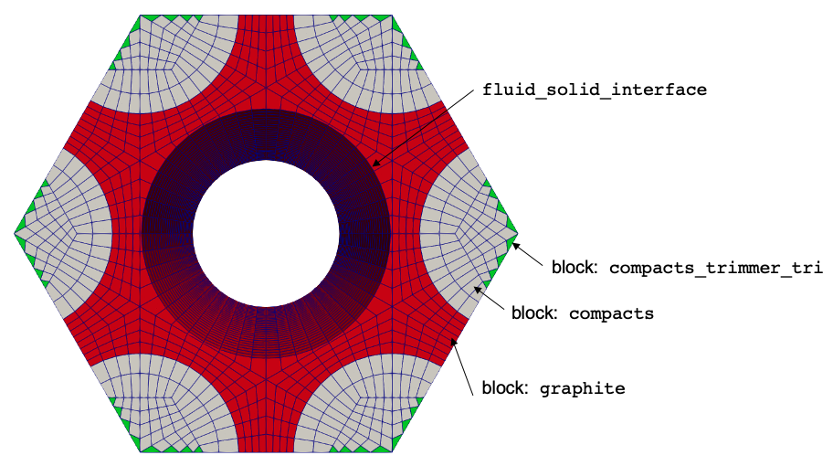
Figure 2: Mesh for the solid heat conduction model
This mesh is generated using MOOSE mesh generators in the mesh.i file.
[Mesh<<<{"href": "../syntax/Mesh/index.html"}>>>]
  [fuel_pin]
    type = PolygonConcentricCircleMeshGenerator<<<{"description": "This PolygonConcentricCircleMeshGenerator object is designed to mesh a polygon geometry with optional rings centered inside.", "href": "../source/meshgenerators/PolygonConcentricCircleMeshGenerator.html"}>>>
    num_sides<<<{"description": "Number of sides of the polygon."}>>> = 6
    polygon_size<<<{"description": "Size of the polygon to be generated (given as either apothem or radius depending on polygon_size_style)."}>>> = '${fparse fuel_to_coolant_distance / 2.0}'
    ring_radii<<<{"description": "Radii of major concentric circles (rings)."}>>> = '${fparse 0.8 * compact_diameter / 2.0} ${fparse compact_diameter / 2.0}'
    ring_intervals<<<{"description": "Number of radial mesh intervals within each major concentric circle excluding their boundary layers."}>>> = '1 1'
    num_sectors_per_side<<<{"description": "Number of azimuthal sectors per polygon side (rotating counterclockwise from top right face)."}>>> = '${ns} ${ns} ${ns} ${ns} ${ns} ${ns}'
    ring_block_ids<<<{"description": "Optional customized block ids for each ring geometry block."}>>> = '2 2'
    ring_block_names<<<{"description": "Optional customized block names for each ring geometry block."}>>> = 'compacts compacts'
    background_block_names<<<{"description": "Optional customized block names for the background block."}>>> = 'graphite'
    background_intervals<<<{"description": "Number of radial meshing intervals in background region (area between rings and ducts) excluding the background's boundary layers."}>>> = 4
  []
  [coolant_pin]
    type = PolygonConcentricCircleMeshGenerator<<<{"description": "This PolygonConcentricCircleMeshGenerator object is designed to mesh a polygon geometry with optional rings centered inside.", "href": "../source/meshgenerators/PolygonConcentricCircleMeshGenerator.html"}>>>
    num_sides<<<{"description": "Number of sides of the polygon."}>>> = 6
    polygon_size<<<{"description": "Size of the polygon to be generated (given as either apothem or radius depending on polygon_size_style)."}>>> = '${fparse fuel_to_coolant_distance / 2.0}'
    ring_radii<<<{"description": "Radii of major concentric circles (rings)."}>>> = '${fparse channel_diameter / 2.0}'
    ring_intervals<<<{"description": "Number of radial mesh intervals within each major concentric circle excluding their boundary layers."}>>> = '2'
    num_sectors_per_side<<<{"description": "Number of azimuthal sectors per polygon side (rotating counterclockwise from top right face)."}>>> = '${ns} ${ns} ${ns} ${ns} ${ns} ${ns}'
    ring_block_ids<<<{"description": "Optional customized block ids for each ring geometry block."}>>> = '101 101'
    ring_block_names<<<{"description": "Optional customized block names for each ring geometry block."}>>> = 'coolant coolant'
    background_block_names<<<{"description": "Optional customized block names for the background block."}>>> = 'graphite'
    interface_boundary_id_shift<<<{"description": "Integer used to shift interface boundary IDs."}>>> = 100
    background_intervals<<<{"description": "Number of radial meshing intervals in background region (area between rings and ducts) excluding the background's boundary layers."}>>> = 1
  []
  [bundle]
    type = PatternedHexMeshGenerator<<<{"description": "This PatternedHexMeshGenerator source code assembles hexagonal meshes into a hexagonal grid and optionally forces the outer boundary to be hexagonal and/or adds a duct.", "href": "../source/meshgenerators/PatternedHexMeshGenerator.html"}>>>
    inputs<<<{"description": "The input MeshGenerators."}>>> = 'fuel_pin coolant_pin'
    hexagon_size<<<{"description": "Size of the outmost hexagon boundary to be generated; this is required only when pattern type is 'hexagon'."}>>> = '${fparse 2.0 * fuel_to_coolant_distance}'
    pattern<<<{"description": "A double-indexed hexagonal-shaped array starting with the upper-left corner."}>>> = '0 0;
              0 1 0;
               0 0'
  []
  [trim]
    type = HexagonMeshTrimmer<<<{"description": "This HexagonMeshTrimmer object performs peripheral and/or across-center (0, 0, 0) trimming for assembly or core 2D meshes generated by PatternedHexMG.", "href": "../source/meshgenerators/HexagonMeshTrimmer.html"}>>>
    input<<<{"description": "The input mesh that needs to be trimmed."}>>> = bundle
    trim_peripheral_region<<<{"description": "Whether the peripheral region on each of the six sides will be trimmed in an assembly mesh. See documentation for numbering convention."}>>> = '1 1 1 1 1 1'
    peripheral_trimming_section_boundary<<<{"description": "Boundary formed by peripheral trimming."}>>> = peripheral_section
  []
  [rotate]
    type = TransformGenerator<<<{"description": "Applies a linear transform to the entire mesh.", "href": "../source/meshgenerators/TransformGenerator.html"}>>>
    input<<<{"description": "The mesh we want to modify"}>>> = trim
    transform<<<{"description": "The type of transformation to perform (TRANSLATE, TRANSLATE_CENTER_ORIGIN, TRANSLATE_MIN_ORIGIN, ROTATE, SCALE, ROTATE_WITH_MATRIX, ROTATE_EXT)"}>>> = rotate
    vector_value<<<{"description": "The value to use for the transformation. When using TRANSLATE or SCALE, the xyz coordinates are applied in each direction respectively. When using ROTATE, the values are interpreted as the Euler angles phi, theta and psi given in degrees. For ROTATE_EXT, an extrinsic rotation is carried out using prescribed Euler angles alpha, beta, and gamma in degrees."}>>> = '30.0 0.0 0.0'
  []
  [extrude]
    type = AdvancedExtruderGenerator<<<{"description": "Extrudes a 1D mesh into 2D, or a 2D mesh into 3D, and supports a variable height for each elevation, variable number of layers within each elevation, variable growth factors of axial element sizes within each elevation and remap subdomain_ids, boundary_ids and element extra integers within each elevation as well as interface boundaries between neighboring elevation layers, as well as following a 1D curve and modifying the radial (normal to the extrusion axis) extent of the geometry.", "href": "../source/meshgenerators/AdvancedExtruderGenerator.html"}>>>
    input<<<{"description": "The mesh to extrude"}>>> = rotate
    heights<<<{"description": "The height of each elevation"}>>> = ${height}
    num_layers<<<{"description": "The number of layers for each elevation - must be num_elevations in length!"}>>> = ${n_layers}
    direction<<<{"description": "A vector that points in the direction to extrude (note, this will be normalized internally - so don't worry about it here)"}>>> = '0 0 1'
  []
  [fluid_solid_interface]
    type = SideSetsBetweenSubdomainsGenerator<<<{"description": "MeshGenerator that creates a sideset composed of the nodes located between two or more subdomains.", "href": "../source/meshgenerators/SideSetsBetweenSubdomainsGenerator.html"}>>>
    input<<<{"description": "The mesh we want to modify"}>>> = extrude
    primary_block<<<{"description": "The primary set of blocks for which to draw a sideset between"}>>> = 'graphite'
    paired_block<<<{"description": "The paired set of blocks for which to draw a sideset between"}>>> = 'coolant'
    new_boundary<<<{"description": "The list of boundary names to create on the supplied subdomain"}>>> = 'fluid_solid_interface'
  []
  [delete_coolant]
    type = BlockDeletionGenerator<<<{"description": "Mesh generator which removes elements from the specified subdomains", "href": "../source/meshgenerators/BlockDeletionGenerator.html"}>>>
    input<<<{"description": "The mesh we want to modify"}>>> = fluid_solid_interface
    block<<<{"description": "The list of blocks to be processed (deleted or kept)"}>>> = 'coolant'
  []
[]We first create a full 7-pin bundle, and then apply a trimming operation to split the compacts. Because MOOSE does not support multiple element types (e.g. tets, hexes) on the same block ID, the trimmer automatically creates an additional block (compacts_trimmer_tri) to represent the triangular prism elements formed in the compacts. You can generate this mesh by running
cardinal-opt -i mesh.i --mesh-only
which will create the mesh, named mesh_in.e.
Because this tutorial only considers temperature coupling, no fluid flow and heat transfer in the helium is modeled. Therefore, heat removal by the fluid is approximated by setting the coolant channel surface to a Dirichlet temperature condition of , where is given as
(2)
where is the fission volumetric power density, is the mass flowrate, is the fluid isobaric specific heat capacity, is the fluid temperature, and is the fluid inlet temperature. Although we will be computing power with OpenMC, just for the sake of applying a fluid temperature boundary condition, we assume the axial power distribution is sinusoidal,
(3)
where is the compact height and is a constant to obtain the total specified power of 30 kW. The nominal fluid mass flowrate is 0.011 kg/s and the inlet temperature is 325°C. All other boundaries in the solid domain are insulated. We will run the OpenMC model first, so the only initial condition required for the solid model is an initial temperature of 325°C.
OpenMC Model
The OpenMC model is built using CSG. The TRISO positions are sampled using the RSA algorithm in OpenMC. OpenMC's Python API is used to create the model with the script shown below. First, we define materials for the various regions. Next, we create a single TRISO particle universe consisting of the five layers of the particle and an infinite extent of graphite filling all other space. We then pack pack uniform-radius spheres into a cylindrical region representing a fuel compact, setting each sphere to be filled with the TRISO universe.
#!/bin/env python

from argparse import ArgumentParser
import math
import numpy as np
import matplotlib.pyplot as plt
import openmc

outlet_P = 7.1e6                         # fluid outlet pressure (Pa)
inlet_T = 598.0                          # inlet fluid temperature (K)
power = 30e3                             # unit cell power (W)
mdot = 0.011                             # fluid mass flowrate (kg/s)
fluid_Cp = 5189.0                        # fluid isobaric specific heat (J/kg/K)
channel_diameter = 0.016                 # diameter of the coolant channels (m)
compact_diameter = 0.0127                # diameter of fuel compacts (m)
fuel_to_coolant_distance = 0.01628       # distance between center of fuel compact and coolant channel (m)
height = 1.60                            # height of the unit cell (m)
triso_pf = 0.15                          # TRISO packing fraction (%)
kernel_radius = 214.85e-6                # fissile kernel outer radius (m)
buffer_radius = 314.85e-6                # buffer outer radius (m)
iPyC_radius = 354.85e-6                  # inner PyC outer radius (m)
SiC_radius = 389.85e-6                   # SiC outer radius (m)
oPyC_radius = 429.85e-6                  # outer PyC outer radius (m)
enrichment = 0.155                       # fuel enrichment (weight percent)
kernel_density = 10820                   # fissile kernel density (kg/m3)
buffer_density = 1050                    # buffer density (kg/m3)
PyC_density = 1900                       # PyC density (kg/m3)
SiC_density = 3203                       # SiC density (kg/m3)
matrix_density = 1700                    # graphite matrix density (kg/m3)

def coolant_temp(t_in, t_out, l, z):
    """
    THIS IS ONLY USED FOR SETTING AN INITIAL CONDITION IN OPENMC's XML FILES -
    the coolant temperature will be applied from MOOSE, we just set an initial
    value here in case you want to run these files in standalone mode (i.e. with
    the "openmc" executable).

    Computes the coolant temperature based on an expected cosine power distribution
    for a specified temperature rise. The total core temperature rise is governed
    by energy conservation as dT = Q / m / Cp, where dT is the total core temperature
    rise, Q is the total core power, m is the mass flowrate, and Cp is the fluid
    isobaric specific heat. If you neglect axial heat conduction and assume steady
    state, then the temperature rise in a layer of fluid i can be related to the
    ratio of the power in that layer to the total power,
    dT_i / dT = Q_i / Q. We assume here a sinusoidal power distribution to get
    a reasonable estimate of an initial coolant temperature distribution.

    Parameters
    ----------

    t_in : float
        Inlet temperature of the channel
    t_out : float
        Outlet temperature of the channel
    l : float
        Length of the channel
    z : float or 1-D numpy.array
        Axial position where the temperature will be computed

    Returns
    -------
        float or 1-D numpy array of float depending on z
    """
    dT = t_out - t_in
    Q = 2 * l / math.pi
    Qi = (l - l * np.cos(math.pi * z / l)) / math.pi

    t = t_in + Qi / Q * dT

    return t

def coolant_density(t):
  """
    THIS IS ONLY USED FOR SETTING AN INITIAL CONDITION IN OPENMC's XML FILES -
    the coolant density will be applied from MOOSE, we just set an initial
    value here in case you want to run these files in standalone mode (i.e. with
    the "openmc" executable).

  Computes the helium density (kg/m3) from temperature assuming a fixed operating pressure.

  Parameters
  ----------

  t : float
    Fluid temperature

  Returns
  _______
    float or 1-D numpy array of float depending on t
  """

  p_in_bar = outlet_P * 1.0e-5
  return 48.14 * p_in_bar / (t + 0.4446 * p_in_bar / math.pow(t, 0.2))

# -------------- Unit Conversions: OpenMC requires cm -----------
m = 100.0
# -------------------------------------------

### RADIANT UNIT CELL SPECS (INFERRED FROM REPORTS) ###

# estimate the outlet temperature using bulk energy conservation for steady state
coolant_outlet_temp = power / mdot / fluid_Cp + inlet_T

# geometry
coolant_channel_diam = channel_diameter * m
reactor_bottom = 0.0
reactor_height = height * m
reactor_top = reactor_bottom + reactor_height

### ARBITRARILY DETERMINED PARAMETERS ###

cell_pitch = fuel_to_coolant_distance * m
fuel_channel_diam = compact_diameter * m

hex_orientation = 'x'

def unit_cell(n_ax_zones, n_inactive, n_active, add_entropy_mesh=False):
    axial_section_height = reactor_height / n_ax_zones

    # superimposed search lattice
    triso_lattice_shape = (4, 4, int(axial_section_height / 0.125))

    lattice_orientation = 'x'
    cell_edge_length = cell_pitch

    model = openmc.model.Model()

    ### Materials ###
    enrichment_234        = 2e-3

    # TRISO Materials

    m_fuel = openmc.Material(name='fuel')
    enrichment_uranium = enrichment
    mass_234 = openmc.data.atomic_mass('U234')
    mass_235 = openmc.data.atomic_mass('U235')
    mass_238 = openmc.data.atomic_mass('U238')

    # number of atoms in one gram of uranium mixture
    n_234 = enrichment_234 / mass_234
    n_235 = enrichment_uranium / mass_235
    n_238 = (1.0 - enrichment_uranium - enrichment_234) / mass_238
    total_n = n_234 + n_235 + n_238

    m_fuel.add_nuclide('U234', n_234 / total_n)
    m_fuel.add_nuclide('U235', n_235 / total_n)
    m_fuel.add_nuclide('U238', n_238 / total_n)
    m_fuel.add_element('C'   , 1.50)
    m_fuel.add_element('O'   , 0.50)
    m_fuel.set_density('kg/m3', kernel_density)
    #
    m_graphite_c_buffer = openmc.Material(name='buffer')
    m_graphite_c_buffer.add_element('C', 1.0)
    m_graphite_c_buffer.add_s_alpha_beta('c_Graphite')
    m_graphite_c_buffer.set_density('kg/m3', buffer_density)
    #
    m_graphite_pyc = openmc.Material(name='pyc')
    m_graphite_pyc.add_element('C', 1.0)
    m_graphite_pyc.add_s_alpha_beta('c_Graphite')
    m_graphite_pyc.set_density('kg/m3', PyC_density)
    #
    m_sic = openmc.Material(name='sic')
    m_sic.add_element('C' , 1.0)
    m_sic.add_element('Si', 1.0)
    m_sic.set_density('kg/m3', SiC_density)

    # Graphite moderator
    m_graphite_matrix = openmc.Material(name='graphite moderator')
    m_graphite_matrix.add_element('C', 1.0)
    m_graphite_matrix.add_s_alpha_beta('c_Graphite')
    m_graphite_matrix.set_density('kg/m3', matrix_density)

    # Coolant
    m_coolant = openmc.Material(name='Helium coolant')
    m_coolant.add_element('He', 1.0, 'ao')

    ### Geometry ###

    # TRISO particle
    radius_pyc_outer       = oPyC_radius * m

    s_fuel             = openmc.Sphere(r=kernel_radius*m)
    s_c_buffer         = openmc.Sphere(r=buffer_radius*m)
    s_pyc_inner        = openmc.Sphere(r=iPyC_radius*m)
    s_sic              = openmc.Sphere(r=SiC_radius*m)
    s_pyc_outer        = openmc.Sphere(r=radius_pyc_outer)
    c_triso_fuel       = openmc.Cell(name='c_triso_fuel'     , fill=m_fuel,              region=-s_fuel)
    c_triso_c_buffer   = openmc.Cell(name='c_triso_c_buffer' , fill=m_graphite_c_buffer, region=+s_fuel      & -s_c_buffer)
    c_triso_pyc_inner  = openmc.Cell(name='c_triso_pyc_inner', fill=m_graphite_pyc,      region=+s_c_buffer  & -s_pyc_inner)
    c_triso_sic        = openmc.Cell(name='c_triso_sic'      , fill=m_sic,               region=+s_pyc_inner & -s_sic)
    c_triso_pyc_outer  = openmc.Cell(name='c_triso_pyc_outer', fill=m_graphite_pyc,      region=+s_sic       & -s_pyc_outer)
    c_triso_matrix     = openmc.Cell(name='c_triso_matrix'   , fill=m_graphite_matrix,   region=+s_pyc_outer)
    u_triso            = openmc.Universe(cells=[c_triso_fuel, c_triso_c_buffer, c_triso_pyc_inner, c_triso_sic, c_triso_pyc_outer, c_triso_matrix])

    # Channel surfaces
    fuel_cyl = openmc.ZCylinder(r=0.5 * fuel_channel_diam)
    coolant_cyl = openmc.ZCylinder(r=0.5 * coolant_channel_diam)

    # create a TRISO lattice for one axial section (to be used in the rest of the axial zones)
    # center the TRISO region on the origin so it fills lattice cells appropriately
    min_z = openmc.ZPlane(z0=-0.5 * axial_section_height)
    max_z = openmc.ZPlane(z0=0.5 * axial_section_height)

    # region in which TRISOs are generated
    r_triso = -fuel_cyl & +min_z & -max_z

    rand_spheres = openmc.model.pack_spheres(radius=radius_pyc_outer, region=r_triso, pf=triso_pf, seed=1.0)
    random_trisos = [openmc.model.TRISO(radius_pyc_outer, u_triso, i) for i in rand_spheres]

    llc, urc = r_triso.bounding_box
    pitch = (urc - llc) / triso_lattice_shape
    # insert TRISOs into a lattice to accelerate point location queries
    triso_lattice = openmc.model.create_triso_lattice(random_trisos, llc, pitch, triso_lattice_shape, m_graphite_matrix)

    # create a hexagonal lattice for the coolant and fuel channels
    fuel_univ = openmc.Universe(cells=[openmc.Cell(region=-fuel_cyl, fill=triso_lattice),
                                    openmc.Cell(region=+fuel_cyl, fill=m_graphite_matrix)])

    # extract the coolant cell and set temperatures based on the axial profile
    coolant_cell = openmc.Cell(region=-coolant_cyl, fill=m_coolant)
    # set the coolant temperature on the cell to approximately match the expected
    # temperature profile
    axial_coords = np.linspace(reactor_bottom, reactor_top, n_ax_zones + 1)
    lattice_univs = []

    fuel_ch_cells = []

    i = 0
    for z_min, z_max in zip(axial_coords[0:-1], axial_coords[1:]):
        # create a new coolant universe for each axial zone in the coolant channel;
        # this generates a new material as well (we only need to do this for all
        # cells except the first cell)
        if (i == 0):
          c_cell = coolant_cell
        else:
          c_cell = coolant_cell.clone()

        i += 1

        # use the middle of the axial section to compute the temperature and density
        ax_pos = 0.5 * (z_min + z_max)
        t = coolant_temp(inlet_T, coolant_outlet_temp, reactor_height, ax_pos)
        c_cell.temperature = t
        coolant_cell.fill.set_density('kg/m3', coolant_density(t))

        # set the solid cells and their temperatures
        graphite_cell = openmc.Cell(region=+coolant_cyl, fill=m_graphite_matrix)
        fuel_ch_cell = openmc.Cell(region=-fuel_cyl, fill=triso_lattice)
        fuel_ch_matrix_cell = openmc.Cell(region=+fuel_cyl, fill=m_graphite_matrix)

        graphite_cell.temperature = t
        fuel_ch_cell.temperature = t
        fuel_ch_matrix_cell.temperature = t

        fuel_ch_cells.append(fuel_ch_cell)
        fuel_u = openmc.Universe(cells=[fuel_ch_cell, fuel_ch_matrix_cell])
        coolant_u = openmc.Universe(cells=[c_cell, graphite_cell])
        lattice_univs.append([[fuel_u] * 6, [coolant_u]])

    # create a hexagonal lattice used in each axial zone to represent the cell
    hex_lattice = openmc.HexLattice(name="Unit cell lattice")
    hex_lattice.orientation = lattice_orientation
    hex_lattice.center = (0.0, 0.0, 0.5 * (reactor_bottom + reactor_top))
    hex_lattice.pitch = (cell_pitch, axial_section_height)
    hex_lattice.universes = lattice_univs

    graphite_outer_cell = openmc.Cell(fill=m_graphite_matrix)
    graphite_outer_cell.temperature = t
    inf_graphite_univ = openmc.Universe(cells=[graphite_outer_cell])
    hex_lattice.outer = inf_graphite_univ

    # hexagonal bounding cell
    hex = openmc.model.HexagonalPrism(cell_edge_length, hex_orientation, boundary_type='periodic')

    hex_cell_vol = 6.0 * (math.sqrt(3) / 4.0) * cell_edge_length**2 * reactor_height

    # create additional axial regions
    axial_planes = [openmc.ZPlane(z0=coord) for coord in axial_coords]
    # axial planes
    min_z = axial_planes[0]
    min_z.boundary_type = 'vacuum'
    max_z = axial_planes[-1]
    max_z.boundary_type = 'vacuum'

    # fill the unit cell with the hex lattice
    hex_cell = openmc.Cell(region=-hex & +min_z & -max_z, fill=hex_lattice)

    model.geometry = openmc.Geometry([hex_cell])

    ### Settings ###
    settings = openmc.Settings()

    settings.particles = 10000
    settings.inactive = n_inactive
    settings.batches = settings.inactive + n_active

    # the only reason we use 'nearest' here is to be sure we have a robust test for CI;
    # otherwise, 1e-16 differences in temperature (due to numerical roundoff when using
    # different MPI ranks) do change the tracking do to the stochastic interpolation
    settings.temperature['method'] = 'nearest'
    settings.temperature['range'] = (294.0, 1500.0)
    settings.temperature['tolerance'] = 200.0

    hexagon_half_flat = math.sqrt(3.0) / 2.0 * cell_edge_length
    lower_left = (-cell_edge_length, -hexagon_half_flat, reactor_bottom)
    upper_right = (cell_edge_length, hexagon_half_flat, reactor_top)
    source_dist = openmc.stats.Box(lower_left, upper_right)
    source = openmc.IndependentSource(space=source_dist)
    settings.source = source

    if (add_entropy_mesh):
      entropy_mesh = openmc.RegularMesh()
      entropy_mesh.lower_left = lower_left
      entropy_mesh.upper_right = upper_right
      entropy_mesh.dimension = (5, 5, 20)
      settings.entropy_mesh = entropy_mesh

    model.settings = settings

    m_colors = {m_coolant: 'royalblue', m_fuel: 'red', m_graphite_c_buffer: 'black', m_graphite_pyc: 'orange', m_sic: 'yellow', m_graphite_matrix: 'silver'}

    plot1          = openmc.Plot()
    plot1.filename = 'plot1'
    plot1.width    = (2 * cell_pitch, 4 * axial_section_height)
    plot1.basis    = 'xz'
    plot1.origin   = (0.0, 0.0, reactor_height/2.0)
    plot1.pixels   = (int(800 * 2 * cell_pitch), int(800 * 4 * axial_section_height))
    plot1.color_by = 'cell'

    plot2          = openmc.Plot()
    plot2.filename = 'plot2'
    plot2.width    = (3 * cell_pitch, 3 * cell_pitch)
    plot2.basis    = 'xy'
    plot2.origin   = (0.0, 0.0, axial_section_height / 2.0)
    plot2.pixels   = (int(800 * cell_pitch), int(800 * cell_pitch))
    plot2.color_by = 'material'
    plot2.colors   = m_colors

    plot3          = openmc.Plot()
    plot3.filename = 'plot3'
    plot3.width    = plot2.width
    plot3.basis    = plot2.basis
    plot3.origin   = plot2.origin
    plot3.pixels   = plot2.pixels
    plot3.color_by = 'cell'

    model.plots = openmc.Plots([plot1, plot2, plot3])

    return model

def main():

    ap = ArgumentParser()
    ap.add_argument('-n', dest='n_axial', type=int, default=30,
                    help='Number of axial cell divisions (defaults to value in common_input.i)')
    ap.add_argument('-s', '--entropy', action='store_true',
                    help='Whether to add a Shannon entropy mesh')
    ap.add_argument('-i', dest='n_inactive', type=int, default=25,
                    help='Number of inactive cycles')
    ap.add_argument('-a', dest='n_active', type=int, default=200,
                    help='Number of active cycles')

    args = ap.parse_args()

    model = unit_cell(args.n_axial, args.n_inactive, args.n_active, args.entropy)
    model.export_to_xml()

if __name__ == "__main__":
    main()
Finally, we loop over axial layers and create unique cells for each of the six compacts, the graphite block, and the coolant. The level on which we will apply feedback from MOOSE is set to 1 because each layer is a component in a lattice nested once with respect to the highest level. To accelerate the particle tracking, we:
Repeat the same TRISO universe in each axial layer and within each compact
Superimpose a Cartesian search lattice in the fuel channel regions.
The OpenMC geometry, colored by cell ID, is shown in Figure 3. The lateral faces of the unit cell are periodic, while the top and bottom boundaries are vacuum. The Cartesian search lattice in the fuel compact regions is also visible.
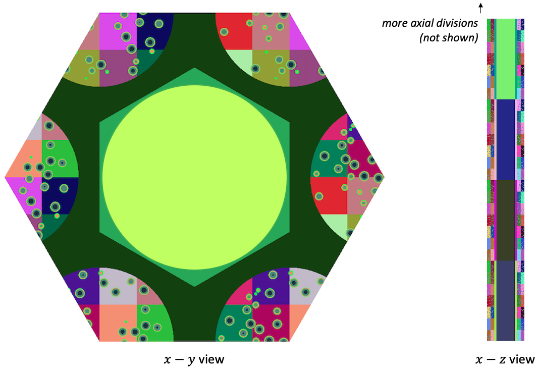
Figure 3: OpenMC model, colored by cell ID
Because we will run OpenMC first, the initial temperature is set to a uniform distribution in the - plane with the axial distribution given by Eq. (2). The fluid density is set using a helium correlation at a fixed pressure of 7.1 MPa Petersen (1970) given the imposed temperature, i.e. .
To create the XML files required to run OpenMC, run the script:
python unit_cell.py
You can also use the XML files checked in to the tutorials/gas_compact directory.
Multiphysics Coupling
In this section, OpenMC and MOOSE are coupled for heat source and temperature feedback for the solid regions of a TRISO-fueled gas reactor compact. The following sub-sections describe these files.
Solid Input Files
The solid phase is solved with the MOOSE heat transfer module, and is described in the solid.i input. We define a number of constants at the beginning of the file and set up the mesh from a file.
compact_diameter = 0.0127                # diameter of fuel compacts (m)
height = 1.60                            # height of the unit cell (m)
triso_pf = 0.15                          # TRISO packing fraction (%)
kernel_radius = 214.85e-6                # fissile kernel outer radius (m)
buffer_radius = 314.85e-6                # buffer outer radius (m)
iPyC_radius = 354.85e-6                  # inner PyC outer radius (m)
SiC_radius = 389.85e-6                   # SiC outer radius (m)
oPyC_radius = 429.85e-6                  # outer PyC outer radius (m)

# material parameters
fluid_Cp = 5189.0                        # fluid isobaric specific heat (J/kg/K)
buffer_k = 0.5                           # buffer thermal conductivity (W/m/K)
PyC_k = 4.0                              # PyC thermal conductivity (W/m/K)
SiC_k = 13.9                             # SiC thermal conductivity (W/m/K)
kernel_k = 3.5                           # fissil kernel thermal conductivity (W/m/K)
matrix_k = 15.0                          # graphite matrix thermal conductivity (W/m/K)

# operating conditions
inlet_T = 598.0                          # inlet fluid temperature (K)
power = 30e3                             # unit cell power (W)
mdot = 0.011                             # fluid mass flowrate (kg/s)

# volume of the fuel compacts (six 1/3-compacts)
compact_vol = ${fparse 2 * pi * compact_diameter * compact_diameter / 4.0 * height}

# compute the volume fraction of each TRISO layer in a TRISO particle
# for use in computing average thermophysical properties
kernel_fraction = ${fparse kernel_radius^3 / oPyC_radius^3}
buffer_fraction = ${fparse (buffer_radius^3 - kernel_radius^3) / oPyC_radius^3}
ipyc_fraction = ${fparse (iPyC_radius^3 - buffer_radius^3) / oPyC_radius^3}
sic_fraction = ${fparse (SiC_radius^3 - iPyC_radius^3) / oPyC_radius^3}
opyc_fraction = ${fparse (oPyC_radius^3 - SiC_radius^3) / oPyC_radius^3}

# multiplicative factor on assumed heat source distribution to get correct magnitude
q0 = ${fparse power / (4.0 * height * compact_diameter * compact_diameter / 4.0)}

[Mesh<<<{"href": "../syntax/Mesh/index.html"}>>>]
  [file]
    type = FileMeshGenerator<<<{"description": "Read a mesh from a file.", "href": "../source/meshgenerators/FileMeshGenerator.html"}>>>
    file<<<{"description": "The filename to read."}>>> = mesh_in.e
  []
[]Next, we define the temperature variable, T, and specify the governing equations and boundary conditions we will apply.
[Variables<<<{"href": "../syntax/Variables/index.html"}>>>]
  [T]
    initial_condition<<<{"description": "Specifies a constant initial condition for this variable"}>>> = ${inlet_T}
  []
[]

[Kernels<<<{"href": "../syntax/Kernels/index.html"}>>>]
  [diffusion]
    type = HeatConduction<<<{"description": "Diffusive heat conduction term $-\\nabla\\cdot(k\\nabla T)$ of the thermal energy conservation equation", "href": "../source/kernels/HeatConduction.html"}>>>
    variable<<<{"description": "The name of the variable that this residual object operates on"}>>> = T
  []
  [source]
    type = CoupledForce<<<{"description": "Implements a source term proportional to the value of a coupled variable. Weak form: $(\\psi_i, -\\sigma v)$.", "href": "../source/kernels/CoupledForce.html"}>>>
    variable<<<{"description": "The name of the variable that this residual object operates on"}>>> = T
    v<<<{"description": "The coupled variable which provides the force"}>>> = power
    block<<<{"description": "The list of blocks (ids or names) that this object will be applied"}>>> = 'compacts compacts_trimmer_tri'
  []
[]

[BCs<<<{"href": "../syntax/BCs/index.html"}>>>]
  [pin_outer]
    type = MatchedValueBC<<<{"description": "Implements a NodalBC which equates two different Variables' values on a specified boundary.", "href": "../source/bcs/MatchedValueBC.html"}>>>
    variable<<<{"description": "The name of the variable that this residual object operates on"}>>> = T
    v<<<{"description": "The variable whose value we are to match."}>>> = fluid_temp
    boundary<<<{"description": "The list of boundary IDs from the mesh where this object applies"}>>> = 'fluid_solid_interface'
  []
[]The MOOSE heat transfer module will receive power from OpenMC in the form of an AuxVariable, so we define a receiver variable for the fission power, as power. We also define a variable fluid_temp, that we will use a FunctionIC to set to the distribution in Eq. (2).
[AuxVariables<<<{"href": "../syntax/AuxVariables/index.html"}>>>]
  [fluid_temp]
  []
  [power]
    family<<<{"description": "Specifies the family of FE shape functions to use for this variable"}>>> = MONOMIAL
    order<<<{"description": "Specifies the order of the FE shape function to use for this variable (additional orders not listed are allowed)"}>>> = CONSTANT
  []
[]

[ICs<<<{"href": "../syntax/Cardinal/ICs/index.html"}>>>]
  [fluid_temp]
    type = FunctionIC<<<{"description": "An initial condition that uses a normal function of x, y, z to produce values (and optionally gradients) for a field variable.", "href": "../source/ics/FunctionIC.html"}>>>
    variable<<<{"description": "The variable this initial condition is supposed to provide values for."}>>> = fluid_temp
    function<<<{"description": "The initial condition function."}>>> = axial_fluid_temp
  []
[]We use functions to define the thermal conductivities and the fluid temperature. The thermal conductivity of the fuel compacts is computed as a volume average of the materials present.
[Functions<<<{"href": "../syntax/Functions/index.html"}>>>]
  [k_graphite]
    type = ParsedFunction<<<{"description": "Function created by parsing a string", "href": "../source/functions/MooseParsedFunction.html"}>>>
    expression<<<{"description": "The user defined function."}>>> = '${matrix_k}'
  []
  [k_TRISO]
    type = ParsedFunction<<<{"description": "Function created by parsing a string", "href": "../source/functions/MooseParsedFunction.html"}>>>
    expression<<<{"description": "The user defined function."}>>> = '${kernel_fraction} * ${kernel_k} + ${buffer_fraction} * ${buffer_k} + ${fparse ipyc_fraction + opyc_fraction} * ${PyC_k} + ${sic_fraction} * ${SiC_k}'
  []
  [k_compacts]
    type = ParsedFunction<<<{"description": "Function created by parsing a string", "href": "../source/functions/MooseParsedFunction.html"}>>>
    expression<<<{"description": "The user defined function."}>>> = '${triso_pf} * k_TRISO + ${fparse 1.0 - triso_pf} * k_graphite'
    symbol_names<<<{"description": "Symbols (excluding t,x,y,z) that are bound to the values provided by the corresponding items in the symbol_values vector."}>>> = 'k_TRISO k_graphite'
    symbol_values<<<{"description": "Constant numeric values, postprocessor names, function names, and scalar variables corresponding to the symbols in symbol_names."}>>> = 'k_TRISO k_graphite'
  []
  [axial_fluid_temp]
    type = ParsedFunction<<<{"description": "Function created by parsing a string", "href": "../source/functions/MooseParsedFunction.html"}>>>
    expression<<<{"description": "The user defined function."}>>> = '${q0} * ${compact_vol} * (${height} - ${height} * cos(pi * z / ${height})) / pi / ${mdot} / ${fluid_Cp} + ${inlet_T}'
  []
[]

[Materials<<<{"href": "../syntax/Materials/index.html"}>>>]
  [graphite]
    type = HeatConductionMaterial<<<{"description": "General-purpose material model for heat conduction", "href": "../source/materials/HeatConductionMaterial.html"}>>>
    thermal_conductivity_temperature_function<<<{"description": "Thermal conductivity as a function of temperature."}>>> = k_graphite
    temp = T
    block<<<{"description": "The list of blocks (ids or names) that this object will be applied"}>>> = 'graphite'
  []
  [compacts]
    type = HeatConductionMaterial<<<{"description": "General-purpose material model for heat conduction", "href": "../source/materials/HeatConductionMaterial.html"}>>>
    thermal_conductivity_temperature_function<<<{"description": "Thermal conductivity as a function of temperature."}>>> = k_compacts
    temp = T
    block<<<{"description": "The list of blocks (ids or names) that this object will be applied"}>>> = 'compacts compacts_trimmer_tri'
  []
[]We define a number of postprocessors for querying the solution as well as for normalizing the fission power, to be described at greater length in Neutronics Input Files .
[Postprocessors<<<{"href": "../syntax/Postprocessors/index.html"}>>>]
  [max_fuel_T]
    type = ElementExtremeValue<<<{"description": "Finds either the min or max elemental value of a variable over the domain.", "href": "../source/postprocessors/ElementExtremeValue.html"}>>>
    variable<<<{"description": "The name of the variable that this postprocessor operates on"}>>> = T
    value_type<<<{"description": "Type of extreme value to return. 'max' returns the maximum value. 'min' returns the minimum value. 'max_abs' returns the maximum of the absolute value."}>>> = max
    block<<<{"description": "The list of blocks (ids or names) that this object will be applied"}>>> = 'compacts compacts_trimmer_tri'
  []
  [max_block_T]
    type = ElementExtremeValue<<<{"description": "Finds either the min or max elemental value of a variable over the domain.", "href": "../source/postprocessors/ElementExtremeValue.html"}>>>
    variable<<<{"description": "The name of the variable that this postprocessor operates on"}>>> = T
    value_type<<<{"description": "Type of extreme value to return. 'max' returns the maximum value. 'min' returns the minimum value. 'max_abs' returns the maximum of the absolute value."}>>> = max
    block<<<{"description": "The list of blocks (ids or names) that this object will be applied"}>>> = 'graphite'
  []
  [power]
    type = ElementIntegralVariablePostprocessor<<<{"description": "Computes a volume integral of the specified variable", "href": "../source/postprocessors/ElementIntegralVariablePostprocessor.html"}>>>
    variable<<<{"description": "The name of the variable that this object operates on"}>>> = power
    block<<<{"description": "The list of blocks (ids or names) that this object will be applied"}>>> = 'compacts compacts_trimmer_tri'
    execute_on<<<{"description": "The list of flag(s) indicating when this object should be executed. For a description of each flag, see https://mooseframework.inl.gov/source/interfaces/SetupInterface.html."}>>> = transfer
  []
[]Even though there are no time-dependent kernels in Eq. (1), we use a Transient such that each Picard iteration between OpenMC and MOOSE heat conduction is essentially one "pseduo" time step ("pseudo" because neither the OpenMC or solid model have any notion of time derivatives).
[Executioner<<<{"href": "../syntax/Executioner/index.html"}>>>]
  type = Transient
  nl_abs_tol = 1e-5
  nl_rel_tol = 1e-16
  petsc_options_value = 'hypre boomeramg'
  petsc_options_iname = '-pc_type -pc_hypre_type'
[]

[Outputs<<<{"href": "../syntax/Outputs/index.html"}>>>]
  exodus<<<{"description": "Output the results using the default settings for Exodus output."}>>> = true
  csv<<<{"description": "Output the scalar variable and postprocessors to a *.csv file using the default CSV output."}>>> = true
  print_linear_residuals<<<{"description": "Enable printing of linear residuals to the screen (Console)"}>>> = false
[]Finally, for additional postprocessing we use a NearestPointLayeredAverage user object to perform averages in the - plane in 30 equal-size layers oriented in the direction. We separate the average by blocks in order to compute separate averages for fuel and graphite temperatures. The layer-wise averages are then exported to the CSV output (in vector postprocessor form) by using two SpatialUserObjectVectorPostprocessors. Note that these user objects are strictly for visualization and generating the plot in Figure 6 - temperatures sent to OpenMC will be taken from the T variable.
[UserObjects<<<{"href": "../syntax/UserObjects/index.html"}>>>]
  [avg_power]
    type = NearestPointLayeredAverage<<<{"description": "Computes averages of a variable storing partial sums for the specified number of intervals in a direction (x,y,z). Given a list of points this object computes the layered average closest to each one of those points.", "href": "../source/userobjects/NearestPointLayeredAverage.html"}>>>
    variable<<<{"description": "The name of the variable that this object operates on"}>>> = heat_source
    points<<<{"description": "Computations will be lumped into values at these points."}>>> = '0.0 0.0 0.0'
    num_layers<<<{"description": "The number of layers."}>>> = 30
    direction<<<{"description": "The direction of the layers."}>>> = z
    block<<<{"description": "The list of block ids (SubdomainID) that this object will be applied"}>>> = 'compacts compacts_trimmer_tri'
  []
  [avg_std_dev]
    type = NearestPointLayeredAverage<<<{"description": "Computes averages of a variable storing partial sums for the specified number of intervals in a direction (x,y,z). Given a list of points this object computes the layered average closest to each one of those points.", "href": "../source/userobjects/NearestPointLayeredAverage.html"}>>>
    variable<<<{"description": "The name of the variable that this object operates on"}>>> = heat_source_std_dev
    points<<<{"description": "Computations will be lumped into values at these points."}>>> = '0.0 0.0 0.0'
    num_layers<<<{"description": "The number of layers."}>>> = 30
    direction<<<{"description": "The direction of the layers."}>>> = z
    block<<<{"description": "The list of block ids (SubdomainID) that this object will be applied"}>>> = 'compacts compacts_trimmer_tri'
  []
[]

[VectorPostprocessors<<<{"href": "../syntax/VectorPostprocessors/index.html"}>>>]
  [avg_q]
    type = SpatialUserObjectVectorPostprocessor<<<{"description": "Outputs the values of a spatial user object in the order of the specified spatial points", "href": "../source/vectorpostprocessors/SpatialUserObjectVectorPostprocessor.html"}>>>
    userobject<<<{"description": "The userobject whose values are to be reported"}>>> = avg_power
  []
  [stdev]
    type = SpatialUserObjectVectorPostprocessor<<<{"description": "Outputs the values of a spatial user object in the order of the specified spatial points", "href": "../source/vectorpostprocessors/SpatialUserObjectVectorPostprocessor.html"}>>>
    userobject<<<{"description": "The userobject whose values are to be reported"}>>> = avg_std_dev
  []
[]Neutronics Input Files
The neutronics physics is solved over the entire domain with OpenMC. The OpenMC wrapping is described in the openmc.i file. We begin by defining a number of constants and by setting up the mesh mirror on which OpenMC will receive temperature from the coupled MOOSE application, and on which OpenMC will write the fission heat source. Because the coupled MOOSE application uses length units of meters, the mesh mirror must also be in units of meters in order to obtain correct data transfers. For simplicity, we just use the same mesh used for solution of the solid heat conduction, though a different mesh could also be used.
height = 1.60                            # height of the unit cell (m)
fluid_Cp = 5189.0                        # fluid isobaric specific heat (J/kg/K)
inlet_T = 598.0                          # inlet fluid temperature (K)
power = 30e3                             # unit cell power (W)
mdot = 0.011                             # fluid mass flowrate (kg/s)

[Mesh<<<{"href": "../syntax/Mesh/index.html"}>>>]
  [solid]
    type = FileMeshGenerator<<<{"description": "Read a mesh from a file.", "href": "../source/meshgenerators/FileMeshGenerator.html"}>>>
    file<<<{"description": "The filename to read."}>>> = mesh_in.e
  []
[]Next, for visualization purposes we define an auxiliary variable and apply a CellTemperatureAux in order to get the temperature imposed on the OpenMC cells. This auxiliary variable will then display the volume-averaged temperature mapped to the OpenMC cells.
[AuxVariables<<<{"href": "../syntax/AuxVariables/index.html"}>>>]
  [cell_temperature]
    family<<<{"description": "Specifies the family of FE shape functions to use for this variable"}>>> = MONOMIAL
    order<<<{"description": "Specifies the order of the FE shape function to use for this variable (additional orders not listed are allowed)"}>>> = CONSTANT
  []
[]

[AuxKernels<<<{"href": "../syntax/AuxKernels/index.html"}>>>]
  [cell_temperature]
    type = CellTemperatureAux<<<{"description": "OpenMC cell temperature (K), mapped to each MOOSE element", "href": "../source/auxkernels/CellTemperatureAux.html"}>>>
    variable<<<{"description": "The name of the variable that this object applies to"}>>> = cell_temperature
  []
[]The [Problem] and [Tallies] blocks are then used to specify settings for the OpenMC wrapping. We define a total power of 30 kW and add a CellTally to the fuel compacts. The cell tally setup in Cardinal will then automatically add a tally for each unique cell ID+instance combination. By setting temperature_blocks to all blocks, OpenMC will then receive temperature from MOOSE for the entire domain (because the mesh mirror consists of these three blocks). Importantly, note that the [Mesh] must always be in units that match the coupled MOOSE application. But because OpenMC solves in units of centimeters, we specify a scaling of 100, i.e. a multiplicative factor to apply to the [Mesh] to get into OpenMC's centimeter units.
[Problem<<<{"href": "../syntax/Problem/index.html"}>>>]
  type = OpenMCCellAverageProblem

  power = ${power}
  scaling = 100.0
  temperature_blocks = 'graphite compacts compacts_trimmer_tri'

  cell_level = 1

  [Tallies<<<{"href": "../syntax/Problem/Tallies/index.html"}>>>]
    [heat_source]
      type = CellTally<<<{"description": "A class which implements distributed cell tallies.", "href": "../source/tallies/CellTally.html"}>>>
      name<<<{"description": "Auxiliary variable name(s) to use for OpenMC tallies. If not specified, defaults to the names of the scores"}>>> = heat_source
      block<<<{"description": "Subdomains for which to add tallies in OpenMC. If not provided, tallies will be applied over the entire domain corresponding to the [Mesh] block."}>>> = 'compacts compacts_trimmer_tri'
      check_equal_mapped_tally_volumes<<<{"description": "Whether to check if the tallied cells map to regions in the mesh of equal volume. This can be helpful to ensure that the volume normalization of OpenMC's tallies doesn't introduce any unintentional distortion just because the mapped volumes are different. You should only set this to true if your OpenMC tally cells are all the same volume!"}>>> = true
      output<<<{"description": "UNRELAXED field(s) to output from OpenMC for each tally score. unrelaxed_tally_std_dev will write the standard deviation of each tally into auxiliary variables named *_std_dev. unrelaxed_tally_rel_error will write the relative standard deviation (unrelaxed_tally_std_dev / unrelaxed_tally) of each tally into auxiliary variables named *_rel_error. unrelaxed_tally will write the raw unrelaxed tally into auxiliary variables named *_raw (replace * with 'name')."}>>> = 'unrelaxed_tally_std_dev'
    []
  []
[]Other features we use include an output of the fission tally standard deviation in units of W/m to the [Mesh] by setting the output parameter. This is used to obtain the standard deviation of the heat source distribution from OpenMC in the same units as the heat source. We also leverage a helper utility in CellTally by setting check_equal_mapped_tally_volumes to true. This parameter will throw an error if the tallied OpenMC cells map to different volumes in the MOOSE domain. Because we know a priori that the equal-volume OpenMC tally cells should all map to equal volumes, this will help ensure that the volumes used for heat source normalization are also all equal. For further discussion of this setting and a pictorial description of the effect of non-equal mapped volumes, please see the OpenMCCellAverageProblem documentation.
Because the OpenMC model is formed by creating axial layers in a lattice nested one level below the highest universe level, the cell level is set to 1. Because the fuel compacts contain TRISO particles, this indicates that all cells in a fuel compact "underneath" level 1 will be set to the same temperature. Because the fuel compacts are homogenized in the heat conduction model, this multiphysics coupling is just an approximation to the true physics. Cardinal supports resolved TRISO multiphysics coupling, provided the solid mesh explicitly resolves the TRISO particles.
Because OpenMC is coupled by temperature to MOOSE, Cardinal automatically adds a variable named temp that will be an intermediate receiver of temperatures from MOOSE (before volume averaging by cell within OpenMCCellAverageProblem). We set an initial condition for temperature in OpenMC by setting a FunctionIC to temp with the function given by Eq. (2).
[ICs<<<{"href": "../syntax/Cardinal/ICs/index.html"}>>>]
  [temp]
    type = FunctionIC<<<{"description": "An initial condition that uses a normal function of x, y, z to produce values (and optionally gradients) for a field variable.", "href": "../source/ics/FunctionIC.html"}>>>
    variable<<<{"description": "The variable this initial condition is supposed to provide values for."}>>> = temp
    function<<<{"description": "The initial condition function."}>>> = temp_ic
  []
[]

[Functions<<<{"href": "../syntax/Functions/index.html"}>>>]
  [temp_ic]
    type = ParsedFunction<<<{"description": "Function created by parsing a string", "href": "../source/functions/MooseParsedFunction.html"}>>>
    expression<<<{"description": "The user defined function."}>>> = '${inlet_T} + z / ${height} * ${power} / ${mdot} / ${fluid_Cp}'
  []
[]We run OpenMC as the main application, so we next need to define a MultiApp that will run the solid heat conduction model as the sub-application. We also require two transfers. To get the fission power into the solid model, we use a MultiAppShapeEvaluationTransfer and ensure conservation of the total power by specifying postprocessors to be preserved in the OpenMC wrapping (heat_source) and in the sub-application (power). To get the temperature into the OpenMC model, we also use a MultiAppShapeEvaluationTransfer in the reverse direction.
[MultiApps<<<{"href": "../syntax/MultiApps/index.html"}>>>]
  [solid]
    type = TransientMultiApp<<<{"description": "MultiApp for performing coupled simulations with the parent and sub-application both progressing in time.", "href": "../source/multiapps/TransientMultiApp.html"}>>>
    input_files<<<{"description": "The input file for each App.  If this parameter only contains one input file it will be used for all of the Apps.  When using 'positions_from_file' it is also admissable to provide one input_file per file."}>>> = 'solid.i'
    execute_on<<<{"description": "The list of flag(s) indicating when this object should be executed. For a description of each flag, see https://mooseframework.inl.gov/source/interfaces/SetupInterface.html."}>>> = timestep_end
  []
[]

[Transfers<<<{"href": "../syntax/Transfers/index.html"}>>>]
  [heat_source_to_solid]
    type = MultiAppGeneralFieldShapeEvaluationTransfer<<<{"description": "Transfers field data at the MultiApp position using the finite element shape functions from the origin application.", "href": "../source/transfers/MultiAppGeneralFieldShapeEvaluationTransfer.html"}>>>
    to_multi_app<<<{"description": "The name of the MultiApp to transfer the data to"}>>> = solid
    variable<<<{"description": "The auxiliary variable to store the transferred values in."}>>> = power
    source_variable<<<{"description": "The variable to transfer from."}>>> = heat_source
    from_postprocessors_to_be_preserved<<<{"description": "The name of the Postprocessor in the from-app to evaluate an adjusting factor."}>>> = heat_source
    to_postprocessors_to_be_preserved<<<{"description": "The name of the Postprocessor in the to-app to evaluate an adjusting factor."}>>> = power
  []
  [temperature_to_openmc]
    type = MultiAppGeneralFieldShapeEvaluationTransfer<<<{"description": "Transfers field data at the MultiApp position using the finite element shape functions from the origin application.", "href": "../source/transfers/MultiAppGeneralFieldShapeEvaluationTransfer.html"}>>>
    from_multi_app<<<{"description": "The name of the MultiApp to receive data from"}>>> = solid
    variable<<<{"description": "The auxiliary variable to store the transferred values in."}>>> = temp
    source_variable<<<{"description": "The variable to transfer from."}>>> = T
  []
[]We define a number of postprocessors to query the solution. The TallyRelativeError extracts the maximum fission tally relative error for monitoring active cycle convergence. The max_power and min_power ElementExtremeValue postprocessors compute the maximum and minimum fission power. And as already discussed, the heat_source postprocessor computes the total power for normalization purposes.
[Postprocessors<<<{"href": "../syntax/Postprocessors/index.html"}>>>]
  [heat_source]
    type = ElementIntegralVariablePostprocessor<<<{"description": "Computes a volume integral of the specified variable", "href": "../source/postprocessors/ElementIntegralVariablePostprocessor.html"}>>>
    variable<<<{"description": "The name of the variable that this object operates on"}>>> = heat_source
    execute_on<<<{"description": "The list of flag(s) indicating when this object should be executed. For a description of each flag, see https://mooseframework.inl.gov/source/interfaces/SetupInterface.html."}>>> = 'transfer initial timestep_end'
    block<<<{"description": "The list of blocks (ids or names) that this object will be applied"}>>> = 'compacts compacts_trimmer_tri'
  []
  [max_tally_rel_err]
    type = TallyRelativeError<<<{"description": "Maximum/minimum tally relative error", "href": "../source/postprocessors/TallyRelativeError.html"}>>>
    value_type<<<{"description": "Whether to give the maximum or minimum tally relative error"}>>> = max
  []
  [max_power]
    type = ElementExtremeValue<<<{"description": "Finds either the min or max elemental value of a variable over the domain.", "href": "../source/postprocessors/ElementExtremeValue.html"}>>>
    variable<<<{"description": "The name of the variable that this postprocessor operates on"}>>> = heat_source
    value_type<<<{"description": "Type of extreme value to return. 'max' returns the maximum value. 'min' returns the minimum value. 'max_abs' returns the maximum of the absolute value."}>>> = max
    block<<<{"description": "The list of blocks (ids or names) that this object will be applied"}>>> = 'compacts compacts_trimmer_tri'
  []
  [min_power]
    type = ElementExtremeValue<<<{"description": "Finds either the min or max elemental value of a variable over the domain.", "href": "../source/postprocessors/ElementExtremeValue.html"}>>>
    variable<<<{"description": "The name of the variable that this postprocessor operates on"}>>> = heat_source
    value_type<<<{"description": "Type of extreme value to return. 'max' returns the maximum value. 'min' returns the minimum value. 'max_abs' returns the maximum of the absolute value."}>>> = min
    block<<<{"description": "The list of blocks (ids or names) that this object will be applied"}>>> = 'compacts compacts_trimmer_tri'
  []
[]We use a NearestPointLayeredAverage to radially average the OpenMC heat source and its standard deviation in axial layers across the 6 compacts. We output the result to CSV using SpatialUserObjectVectorPostprocessors. Note that this user object is strictly used for visualization purposes to generate the plot in Figure 4 - the heat source applied to the MOOSE heat conduction model is taken from the heat_source variable transferred with the heat_source_to_solid transfer.
[UserObjects<<<{"href": "../syntax/UserObjects/index.html"}>>>]
  [avg_power]
    type = NearestPointLayeredAverage<<<{"description": "Computes averages of a variable storing partial sums for the specified number of intervals in a direction (x,y,z). Given a list of points this object computes the layered average closest to each one of those points.", "href": "../source/userobjects/NearestPointLayeredAverage.html"}>>>
    variable<<<{"description": "The name of the variable that this object operates on"}>>> = heat_source
    points<<<{"description": "Computations will be lumped into values at these points."}>>> = '0.0 0.0 0.0'
    num_layers<<<{"description": "The number of layers."}>>> = 30
    direction<<<{"description": "The direction of the layers."}>>> = z
    block<<<{"description": "The list of block ids (SubdomainID) that this object will be applied"}>>> = 'compacts compacts_trimmer_tri'
  []
  [avg_std_dev]
    type = NearestPointLayeredAverage<<<{"description": "Computes averages of a variable storing partial sums for the specified number of intervals in a direction (x,y,z). Given a list of points this object computes the layered average closest to each one of those points.", "href": "../source/userobjects/NearestPointLayeredAverage.html"}>>>
    variable<<<{"description": "The name of the variable that this object operates on"}>>> = heat_source_std_dev
    points<<<{"description": "Computations will be lumped into values at these points."}>>> = '0.0 0.0 0.0'
    num_layers<<<{"description": "The number of layers."}>>> = 30
    direction<<<{"description": "The direction of the layers."}>>> = z
    block<<<{"description": "The list of block ids (SubdomainID) that this object will be applied"}>>> = 'compacts compacts_trimmer_tri'
  []
[]

[VectorPostprocessors<<<{"href": "../syntax/VectorPostprocessors/index.html"}>>>]
  [avg_q]
    type = SpatialUserObjectVectorPostprocessor<<<{"description": "Outputs the values of a spatial user object in the order of the specified spatial points", "href": "../source/vectorpostprocessors/SpatialUserObjectVectorPostprocessor.html"}>>>
    userobject<<<{"description": "The userobject whose values are to be reported"}>>> = avg_power
  []
  [stdev]
    type = SpatialUserObjectVectorPostprocessor<<<{"description": "Outputs the values of a spatial user object in the order of the specified spatial points", "href": "../source/vectorpostprocessors/SpatialUserObjectVectorPostprocessor.html"}>>>
    userobject<<<{"description": "The userobject whose values are to be reported"}>>> = avg_std_dev
  []
[]This input will run OpenMC and the MOOSE heat conduction model in Picard iterations via pseudo time-stepping. We specify a fixed number of time steps by running OpenMC with a Transient executioner. Finally, we specify Exodus and CSV output formats. Note, only four Picard iterations are shown here, but generally, more will be necessary to converge the physics.
[Executioner<<<{"href": "../syntax/Executioner/index.html"}>>>]
  type = Transient
  num_steps = 4
[]

[Outputs<<<{"href": "../syntax/Outputs/index.html"}>>>]
  exodus<<<{"description": "Output the results using the default settings for Exodus output."}>>> = true
  csv<<<{"description": "Output the scalar variable and postprocessors to a *.csv file using the default CSV output."}>>> = true
[]Execution and Postprocessing
To run the coupled calculation,
mpiexec -np 2 cardinal-opt -i openmc.i --n-threads=2
This will run both MOOSE and OpenMC with 2 MPI processes and 2 OpenMP threads per rank. When the simulation has completed, you will have created a number of different output files:
openmc_out.e, an Exodus file with the OpenMC solution and the data that was ultimately transferred in/out of OpenMCopenmc_out_solid0.e, an Exodus file with the solid solutionopenmc_out.csv, a CSV output with the postprocessors fromopenmc.iopenmc_out_solid0.csv, a CSV output with the postprocessors fromsolid.iopenmc_out_avg_q_<n>.csv, CSV output at time step<n>with the radially-averaged fission poweropenmc_out_stdev_<n>.csv, CSV output at time step<n>with the radially-averaged fission power standard deviationopenmc_out_solid0_block_axial_avg_<n>.csv, CSV output at time step<n>with the radially-average block temperatureopenmc_out_solid0_fuel_axial_avg_<n>.csv, CSV output at time step<n>with the radially-average fuel temperature
First, let's examine how the mapping between OpenMC and MOOSE was established. When we run with verbose = true, you will see the following mapping information displayed:
------------------------------------------------------------------------------------
| Cell | Solid | Fluid | Other | Mapped Vol | Actual Vol |
------------------------------------------------------------------------------------
| 11543, instance 0 (of 1) | 48 | 0 | 0 | 1.443e-06 | |
| 11544, instance 0 (of 6) | 68 | 0 | 0 | 2.252e-06 | |
| 11544, instance 1 (of 6) | 68 | 0 | 0 | 2.252e-06 | |
| 11544, instance 2 (of 6) | 68 | 0 | 0 | 2.252e-06 | |
| 11544, instance 3 (of 6) | 68 | 0 | 0 | 2.252e-06 | |
| 11544, instance 4 (of 6) | 68 | 0 | 0 | 2.252e-06 | |
| 11544, instance 5 (of 6) | 68 | 0 | 0 | 2.252e-06 | |
| 11545, instance 0 (of 6) | 64 | 0 | 0 | 1.803e-06 | |
| 11545, instance 1 (of 6) | 64 | 0 | 0 | 1.803e-06 | |
| 11545, instance 2 (of 6) | 64 | 0 | 0 | 1.803e-06 | |
| 11545, instance 3 (of 6) | 64 | 0 | 0 | 1.803e-06 | |
| 11545, instance 4 (of 6) | 64 | 0 | 0 | 1.803e-06 | |
| 11545, instance 5 (of 6) | 64 | 0 | 0 | 1.803e-06 | |
| 11547, instance 0 (of 1) | 48 | 0 | 0 | 1.443e-06 | |
| 11548, instance 0 (of 6) | 68 | 0 | 0 | 2.252e-06 | |
| 11548, instance 1 (of 6) | 68 | 0 | 0 | 2.252e-06 | |
| 11548, instance 2 (of 6) | 68 | 0 | 0 | 2.252e-06 | |
| 11548, instance 3 (of 6) | 68 | 0 | 0 | 2.252e-06 | |
| 11548, instance 4 (of 6) | 68 | 0 | 0 | 2.252e-06 | |
| 11548, instance 5 (of 6) | 68 | 0 | 0 | 2.252e-06 | |
| 11549, instance 0 (of 6) | 64 | 0 | 0 | 1.803e-06 | |
| 11549, instance 1 (of 6) | 64 | 0 | 0 | 1.803e-06 | |
| 11549, instance 2 (of 6) | 64 | 0 | 0 | 1.803e-06 | |
| 11549, instance 3 (of 6) | 64 | 0 | 0 | 1.803e-06 | |
| 11549, instance 4 (of 6) | 64 | 0 | 0 | 1.803e-06 | |
| 11549, instance 5 (of 6) | 64 | 0 | 0 | 1.803e-06 | |
| 11551, instance 0 (of 1) | 48 | 0 | 0 | 1.443e-06 | |
| 11552, instance 0 (of 6) | 68 | 0 | 0 | 2.252e-06 | |
| 11552, instance 1 (of 6) | 68 | 0 | 0 | 2.252e-06 | |
| 11552, instance 2 (of 6) | 68 | 0 | 0 | 2.252e-06 | |
| 11552, instance 3 (of 6) | 68 | 0 | 0 | 2.252e-06 | |
| 11552, instance 4 (of 6) | 68 | 0 | 0 | 2.252e-06 | |
| 11552, instance 5 (of 6) | 68 | 0 | 0 | 2.252e-06 | |
| 11553, instance 0 (of 6) | 64 | 0 | 0 | 1.803e-06 | |
| 11553, instance 1 (of 6) | 64 | 0 | 0 | 1.803e-06 | |
| 11553, instance 2 (of 6) | 64 | 0 | 0 | 1.803e-06 | |
| 11553, instance 3 (of 6) | 64 | 0 | 0 | 1.803e-06 | |
| 11553, instance 4 (of 6) | 64 | 0 | 0 | 1.803e-06 | |
| 11553, instance 5 (of 6) | 64 | 0 | 0 | 1.803e-06 | |
| 11555, instance 0 (of 1) | 48 | 0 | 0 | 1.443e-06 | |
| 11556, instance 0 (of 6) | 68 | 0 | 0 | 2.252e-06 | |
| 11556, instance 1 (of 6) | 68 | 0 | 0 | 2.252e-06 | |
| 11556, instance 2 (of 6) | 68 | 0 | 0 | 2.252e-06 | |
| 11556, instance 3 (of 6) | 68 | 0 | 0 | 2.252e-06 | |
| 11556, instance 4 (of 6) | 68 | 0 | 0 | 2.252e-06 | |
| 11556, instance 5 (of 6) | 68 | 0 | 0 | 2.252e-06 | |
| 11557, instance 0 (of 6) | 64 | 0 | 0 | 1.803e-06 | |
| 11557, instance 1 (of 6) | 64 | 0 | 0 | 1.803e-06 | |
| 11557, instance 2 (of 6) | 64 | 0 | 0 | 1.803e-06 | |
| 11557, instance 3 (of 6) | 64 | 0 | 0 | 1.803e-06 | |
| 11557, instance 4 (of 6) | 64 | 0 | 0 | 1.803e-06 | |
| 11557, instance 5 (of 6) | 64 | 0 | 0 | 1.803e-06 | |
| 11559, instance 0 (of 1) | 48 | 0 | 0 | 1.443e-06 | |
| 11560, instance 0 (of 6) | 68 | 0 | 0 | 2.252e-06 | |
| 11560, instance 1 (of 6) | 68 | 0 | 0 | 2.252e-06 | |
| 11560, instance 2 (of 6) | 68 | 0 | 0 | 2.252e-06 | |
| 11560, instance 3 (of 6) | 68 | 0 | 0 | 2.252e-06 | |
| 11560, instance 4 (of 6) | 68 | 0 | 0 | 2.252e-06 | |
| 11560, instance 5 (of 6) | 68 | 0 | 0 | 2.252e-06 | |
| 11561, instance 0 (of 6) | 64 | 0 | 0 | 1.803e-06 | |
| 11561, instance 1 (of 6) | 64 | 0 | 0 | 1.803e-06 | |
| 11561, instance 2 (of 6) | 64 | 0 | 0 | 1.803e-06 | |
| 11561, instance 3 (of 6) | 64 | 0 | 0 | 1.803e-06 | |
| 11561, instance 4 (of 6) | 64 | 0 | 0 | 1.803e-06 | |
| 11561, instance 5 (of 6) | 64 | 0 | 0 | 1.803e-06 | |
| 11563, instance 0 (of 1) | 48 | 0 | 0 | 1.443e-06 | |
| 11564, instance 0 (of 6) | 68 | 0 | 0 | 2.252e-06 | |
| 11564, instance 1 (of 6) | 68 | 0 | 0 | 2.252e-06 | |
| 11564, instance 2 (of 6) | 68 | 0 | 0 | 2.252e-06 | |
| 11564, instance 3 (of 6) | 68 | 0 | 0 | 2.252e-06 | |
| 11564, instance 4 (of 6) | 68 | 0 | 0 | 2.252e-06 | |
| 11564, instance 5 (of 6) | 68 | 0 | 0 | 2.252e-06 | |
| 11565, instance 0 (of 6) | 64 | 0 | 0 | 1.803e-06 | |
| 11565, instance 1 (of 6) | 64 | 0 | 0 | 1.803e-06 | |
| 11565, instance 2 (of 6) | 64 | 0 | 0 | 1.803e-06 | |
| 11565, instance 3 (of 6) | 64 | 0 | 0 | 1.803e-06 | |
| 11565, instance 4 (of 6) | 64 | 0 | 0 | 1.803e-06 | |
| 11565, instance 5 (of 6) | 64 | 0 | 0 | 1.803e-06 | |
| 11567, instance 0 (of 1) | 48 | 0 | 0 | 1.443e-06 | |
| 11568, instance 0 (of 6) | 68 | 0 | 0 | 2.252e-06 | |
| 11568, instance 1 (of 6) | 68 | 0 | 0 | 2.252e-06 | |
| 11568, instance 2 (of 6) | 68 | 0 | 0 | 2.252e-06 | |
| 11568, instance 3 (of 6) | 68 | 0 | 0 | 2.252e-06 | |
| 11568, instance 4 (of 6) | 68 | 0 | 0 | 2.252e-06 | |
| 11568, instance 5 (of 6) | 68 | 0 | 0 | 2.252e-06 | |
| 11569, instance 0 (of 6) | 64 | 0 | 0 | 1.803e-06 | |
| 11569, instance 1 (of 6) | 64 | 0 | 0 | 1.803e-06 | |
| 11569, instance 2 (of 6) | 64 | 0 | 0 | 1.803e-06 | |
| 11569, instance 3 (of 6) | 64 | 0 | 0 | 1.803e-06 | |
| 11569, instance 4 (of 6) | 64 | 0 | 0 | 1.803e-06 | |
| 11569, instance 5 (of 6) | 64 | 0 | 0 | 1.803e-06 | |
| 11571, instance 0 (of 1) | 48 | 0 | 0 | 1.443e-06 | |
| 11572, instance 0 (of 6) | 68 | 0 | 0 | 2.252e-06 | |
| 11572, instance 1 (of 6) | 68 | 0 | 0 | 2.252e-06 | |
| 11572, instance 2 (of 6) | 68 | 0 | 0 | 2.252e-06 | |
| 11572, instance 3 (of 6) | 68 | 0 | 0 | 2.252e-06 | |
| 11572, instance 4 (of 6) | 68 | 0 | 0 | 2.252e-06 | |
| 11572, instance 5 (of 6) | 68 | 0 | 0 | 2.252e-06 | |
| 11573, instance 0 (of 6) | 64 | 0 | 0 | 1.803e-06 | |
| 11573, instance 1 (of 6) | 64 | 0 | 0 | 1.803e-06 | |
| 11573, instance 2 (of 6) | 64 | 0 | 0 | 1.803e-06 | |
| 11573, instance 3 (of 6) | 64 | 0 | 0 | 1.803e-06 | |
| 11573, instance 4 (of 6) | 64 | 0 | 0 | 1.803e-06 | |
| 11573, instance 5 (of 6) | 64 | 0 | 0 | 1.803e-06 | |
| 11575, instance 0 (of 1) | 48 | 0 | 0 | 1.443e-06 | |
| 11576, instance 0 (of 6) | 68 | 0 | 0 | 2.252e-06 | |
| 11576, instance 1 (of 6) | 68 | 0 | 0 | 2.252e-06 | |
| 11576, instance 2 (of 6) | 68 | 0 | 0 | 2.252e-06 | |
| 11576, instance 3 (of 6) | 68 | 0 | 0 | 2.252e-06 | |
| 11576, instance 4 (of 6) | 68 | 0 | 0 | 2.252e-06 | |
| 11576, instance 5 (of 6) | 68 | 0 | 0 | 2.252e-06 | |
| 11577, instance 0 (of 6) | 64 | 0 | 0 | 1.803e-06 | |
| 11577, instance 1 (of 6) | 64 | 0 | 0 | 1.803e-06 | |
| 11577, instance 2 (of 6) | 64 | 0 | 0 | 1.803e-06 | |
| 11577, instance 3 (of 6) | 64 | 0 | 0 | 1.803e-06 | |
| 11577, instance 4 (of 6) | 64 | 0 | 0 | 1.803e-06 | |
| 11577, instance 5 (of 6) | 64 | 0 | 0 | 1.803e-06 | |
| 11579, instance 0 (of 1) | 48 | 0 | 0 | 1.443e-06 | |
| 11580, instance 0 (of 6) | 68 | 0 | 0 | 2.252e-06 | |
| 11580, instance 1 (of 6) | 68 | 0 | 0 | 2.252e-06 | |
| 11580, instance 2 (of 6) | 68 | 0 | 0 | 2.252e-06 | |
| 11580, instance 3 (of 6) | 68 | 0 | 0 | 2.252e-06 | |
| 11580, instance 4 (of 6) | 68 | 0 | 0 | 2.252e-06 | |
| 11580, instance 5 (of 6) | 68 | 0 | 0 | 2.252e-06 | |
| 11581, instance 0 (of 6) | 64 | 0 | 0 | 1.803e-06 | |
| 11581, instance 1 (of 6) | 64 | 0 | 0 | 1.803e-06 | |
| 11581, instance 2 (of 6) | 64 | 0 | 0 | 1.803e-06 | |
| 11581, instance 3 (of 6) | 64 | 0 | 0 | 1.803e-06 | |
| 11581, instance 4 (of 6) | 64 | 0 | 0 | 1.803e-06 | |
| 11581, instance 5 (of 6) | 64 | 0 | 0 | 1.803e-06 | |
| 11583, instance 0 (of 1) | 48 | 0 | 0 | 1.443e-06 | |
| 11584, instance 0 (of 6) | 68 | 0 | 0 | 2.252e-06 | |
| 11584, instance 1 (of 6) | 68 | 0 | 0 | 2.252e-06 | |
| 11584, instance 2 (of 6) | 68 | 0 | 0 | 2.252e-06 | |
| 11584, instance 3 (of 6) | 68 | 0 | 0 | 2.252e-06 | |
| 11584, instance 4 (of 6) | 68 | 0 | 0 | 2.252e-06 | |
| 11584, instance 5 (of 6) | 68 | 0 | 0 | 2.252e-06 | |
| 11585, instance 0 (of 6) | 64 | 0 | 0 | 1.803e-06 | |
| 11585, instance 1 (of 6) | 64 | 0 | 0 | 1.803e-06 | |
| 11585, instance 2 (of 6) | 64 | 0 | 0 | 1.803e-06 | |
| 11585, instance 3 (of 6) | 64 | 0 | 0 | 1.803e-06 | |
| 11585, instance 4 (of 6) | 64 | 0 | 0 | 1.803e-06 | |
| 11585, instance 5 (of 6) | 64 | 0 | 0 | 1.803e-06 | |
| 11587, instance 0 (of 1) | 48 | 0 | 0 | 1.443e-06 | |
| 11588, instance 0 (of 6) | 68 | 0 | 0 | 2.252e-06 | |
| 11588, instance 1 (of 6) | 68 | 0 | 0 | 2.252e-06 | |
| 11588, instance 2 (of 6) | 68 | 0 | 0 | 2.252e-06 | |
| 11588, instance 3 (of 6) | 68 | 0 | 0 | 2.252e-06 | |
| 11588, instance 4 (of 6) | 68 | 0 | 0 | 2.252e-06 | |
| 11588, instance 5 (of 6) | 68 | 0 | 0 | 2.252e-06 | |
| 11589, instance 0 (of 6) | 64 | 0 | 0 | 1.803e-06 | |
| 11589, instance 1 (of 6) | 64 | 0 | 0 | 1.803e-06 | |
| 11589, instance 2 (of 6) | 64 | 0 | 0 | 1.803e-06 | |
| 11589, instance 3 (of 6) | 64 | 0 | 0 | 1.803e-06 | |
| 11589, instance 4 (of 6) | 64 | 0 | 0 | 1.803e-06 | |
| 11589, instance 5 (of 6) | 64 | 0 | 0 | 1.803e-06 | |
| 11591, instance 0 (of 1) | 48 | 0 | 0 | 1.443e-06 | |
| 11592, instance 0 (of 6) | 68 | 0 | 0 | 2.252e-06 | |
| 11592, instance 1 (of 6) | 68 | 0 | 0 | 2.252e-06 | |
| 11592, instance 2 (of 6) | 68 | 0 | 0 | 2.252e-06 | |
| 11592, instance 3 (of 6) | 68 | 0 | 0 | 2.252e-06 | |
| 11592, instance 4 (of 6) | 68 | 0 | 0 | 2.252e-06 | |
| 11592, instance 5 (of 6) | 68 | 0 | 0 | 2.252e-06 | |
| 11593, instance 0 (of 6) | 64 | 0 | 0 | 1.803e-06 | |
| 11593, instance 1 (of 6) | 64 | 0 | 0 | 1.803e-06 | |
| 11593, instance 2 (of 6) | 64 | 0 | 0 | 1.803e-06 | |
| 11593, instance 3 (of 6) | 64 | 0 | 0 | 1.803e-06 | |
| 11593, instance 4 (of 6) | 64 | 0 | 0 | 1.803e-06 | |
| 11593, instance 5 (of 6) | 64 | 0 | 0 | 1.803e-06 | |
| 11595, instance 0 (of 1) | 48 | 0 | 0 | 1.443e-06 | |
| 11596, instance 0 (of 6) | 68 | 0 | 0 | 2.252e-06 | |
| 11596, instance 1 (of 6) | 68 | 0 | 0 | 2.252e-06 | |
| 11596, instance 2 (of 6) | 68 | 0 | 0 | 2.252e-06 | |
| 11596, instance 3 (of 6) | 68 | 0 | 0 | 2.252e-06 | |
| 11596, instance 4 (of 6) | 68 | 0 | 0 | 2.252e-06 | |
| 11596, instance 5 (of 6) | 68 | 0 | 0 | 2.252e-06 | |
| 11597, instance 0 (of 6) | 64 | 0 | 0 | 1.803e-06 | |
| 11597, instance 1 (of 6) | 64 | 0 | 0 | 1.803e-06 | |
| 11597, instance 2 (of 6) | 64 | 0 | 0 | 1.803e-06 | |
| 11597, instance 3 (of 6) | 64 | 0 | 0 | 1.803e-06 | |
| 11597, instance 4 (of 6) | 64 | 0 | 0 | 1.803e-06 | |
| 11597, instance 5 (of 6) | 64 | 0 | 0 | 1.803e-06 | |
| 11599, instance 0 (of 1) | 48 | 0 | 0 | 1.443e-06 | |
| 11600, instance 0 (of 6) | 68 | 0 | 0 | 2.252e-06 | |
| 11600, instance 1 (of 6) | 68 | 0 | 0 | 2.252e-06 | |
| 11600, instance 2 (of 6) | 68 | 0 | 0 | 2.252e-06 | |
| 11600, instance 3 (of 6) | 68 | 0 | 0 | 2.252e-06 | |
| 11600, instance 4 (of 6) | 68 | 0 | 0 | 2.252e-06 | |
| 11600, instance 5 (of 6) | 68 | 0 | 0 | 2.252e-06 | |
| 11601, instance 0 (of 6) | 64 | 0 | 0 | 1.803e-06 | |
| 11601, instance 1 (of 6) | 64 | 0 | 0 | 1.803e-06 | |
| 11601, instance 2 (of 6) | 64 | 0 | 0 | 1.803e-06 | |
| 11601, instance 3 (of 6) | 64 | 0 | 0 | 1.803e-06 | |
| 11601, instance 4 (of 6) | 64 | 0 | 0 | 1.803e-06 | |
| 11601, instance 5 (of 6) | 64 | 0 | 0 | 1.803e-06 | |
| 11603, instance 0 (of 1) | 48 | 0 | 0 | 1.443e-06 | |
| 11604, instance 0 (of 6) | 68 | 0 | 0 | 2.252e-06 | |
| 11604, instance 1 (of 6) | 68 | 0 | 0 | 2.252e-06 | |
| 11604, instance 2 (of 6) | 68 | 0 | 0 | 2.252e-06 | |
| 11604, instance 3 (of 6) | 68 | 0 | 0 | 2.252e-06 | |
| 11604, instance 4 (of 6) | 68 | 0 | 0 | 2.252e-06 | |
| 11604, instance 5 (of 6) | 68 | 0 | 0 | 2.252e-06 | |
| 11605, instance 0 (of 6) | 64 | 0 | 0 | 1.803e-06 | |
| 11605, instance 1 (of 6) | 64 | 0 | 0 | 1.803e-06 | |
| 11605, instance 2 (of 6) | 64 | 0 | 0 | 1.803e-06 | |
| 11605, instance 3 (of 6) | 64 | 0 | 0 | 1.803e-06 | |
| 11605, instance 4 (of 6) | 64 | 0 | 0 | 1.803e-06 | |
| 11605, instance 5 (of 6) | 64 | 0 | 0 | 1.803e-06 | |
| 11607, instance 0 (of 1) | 48 | 0 | 0 | 1.443e-06 | |
| 11608, instance 0 (of 6) | 68 | 0 | 0 | 2.252e-06 | |
| 11608, instance 1 (of 6) | 68 | 0 | 0 | 2.252e-06 | |
| 11608, instance 2 (of 6) | 68 | 0 | 0 | 2.252e-06 | |
| 11608, instance 3 (of 6) | 68 | 0 | 0 | 2.252e-06 | |
| 11608, instance 4 (of 6) | 68 | 0 | 0 | 2.252e-06 | |
| 11608, instance 5 (of 6) | 68 | 0 | 0 | 2.252e-06 | |
| 11609, instance 0 (of 6) | 64 | 0 | 0 | 1.803e-06 | |
| 11609, instance 1 (of 6) | 64 | 0 | 0 | 1.803e-06 | |
| 11609, instance 2 (of 6) | 64 | 0 | 0 | 1.803e-06 | |
| 11609, instance 3 (of 6) | 64 | 0 | 0 | 1.803e-06 | |
| 11609, instance 4 (of 6) | 64 | 0 | 0 | 1.803e-06 | |
| 11609, instance 5 (of 6) | 64 | 0 | 0 | 1.803e-06 | |
| 11611, instance 0 (of 1) | 48 | 0 | 0 | 1.443e-06 | |
| 11612, instance 0 (of 6) | 68 | 0 | 0 | 2.252e-06 | |
| 11612, instance 1 (of 6) | 68 | 0 | 0 | 2.252e-06 | |
| 11612, instance 2 (of 6) | 68 | 0 | 0 | 2.252e-06 | |
| 11612, instance 3 (of 6) | 68 | 0 | 0 | 2.252e-06 | |
| 11612, instance 4 (of 6) | 68 | 0 | 0 | 2.252e-06 | |
| 11612, instance 5 (of 6) | 68 | 0 | 0 | 2.252e-06 | |
| 11613, instance 0 (of 6) | 64 | 0 | 0 | 1.803e-06 | |
| 11613, instance 1 (of 6) | 64 | 0 | 0 | 1.803e-06 | |
| 11613, instance 2 (of 6) | 64 | 0 | 0 | 1.803e-06 | |
| 11613, instance 3 (of 6) | 64 | 0 | 0 | 1.803e-06 | |
| 11613, instance 4 (of 6) | 64 | 0 | 0 | 1.803e-06 | |
| 11613, instance 5 (of 6) | 64 | 0 | 0 | 1.803e-06 | |
| 11615, instance 0 (of 1) | 48 | 0 | 0 | 1.443e-06 | |
| 11616, instance 0 (of 6) | 68 | 0 | 0 | 2.252e-06 | |
| 11616, instance 1 (of 6) | 68 | 0 | 0 | 2.252e-06 | |
| 11616, instance 2 (of 6) | 68 | 0 | 0 | 2.252e-06 | |
| 11616, instance 3 (of 6) | 68 | 0 | 0 | 2.252e-06 | |
| 11616, instance 4 (of 6) | 68 | 0 | 0 | 2.252e-06 | |
| 11616, instance 5 (of 6) | 68 | 0 | 0 | 2.252e-06 | |
| 11617, instance 0 (of 6) | 64 | 0 | 0 | 1.803e-06 | |
| 11617, instance 1 (of 6) | 64 | 0 | 0 | 1.803e-06 | |
| 11617, instance 2 (of 6) | 64 | 0 | 0 | 1.803e-06 | |
| 11617, instance 3 (of 6) | 64 | 0 | 0 | 1.803e-06 | |
| 11617, instance 4 (of 6) | 64 | 0 | 0 | 1.803e-06 | |
| 11617, instance 5 (of 6) | 64 | 0 | 0 | 1.803e-06 | |
| 11619, instance 0 (of 1) | 48 | 0 | 0 | 1.443e-06 | |
| 11620, instance 0 (of 6) | 68 | 0 | 0 | 2.252e-06 | |
| 11620, instance 1 (of 6) | 68 | 0 | 0 | 2.252e-06 | |
| 11620, instance 2 (of 6) | 68 | 0 | 0 | 2.252e-06 | |
| 11620, instance 3 (of 6) | 68 | 0 | 0 | 2.252e-06 | |
| 11620, instance 4 (of 6) | 68 | 0 | 0 | 2.252e-06 | |
| 11620, instance 5 (of 6) | 68 | 0 | 0 | 2.252e-06 | |
| 11621, instance 0 (of 6) | 64 | 0 | 0 | 1.803e-06 | |
| 11621, instance 1 (of 6) | 64 | 0 | 0 | 1.803e-06 | |
| 11621, instance 2 (of 6) | 64 | 0 | 0 | 1.803e-06 | |
| 11621, instance 3 (of 6) | 64 | 0 | 0 | 1.803e-06 | |
| 11621, instance 4 (of 6) | 64 | 0 | 0 | 1.803e-06 | |
| 11621, instance 5 (of 6) | 64 | 0 | 0 | 1.803e-06 | |
| 11623, instance 0 (of 1) | 48 | 0 | 0 | 1.443e-06 | |
| 11624, instance 0 (of 6) | 68 | 0 | 0 | 2.252e-06 | |
| 11624, instance 1 (of 6) | 68 | 0 | 0 | 2.252e-06 | |
| 11624, instance 2 (of 6) | 68 | 0 | 0 | 2.252e-06 | |
| 11624, instance 3 (of 6) | 68 | 0 | 0 | 2.252e-06 | |
| 11624, instance 4 (of 6) | 68 | 0 | 0 | 2.252e-06 | |
| 11624, instance 5 (of 6) | 68 | 0 | 0 | 2.252e-06 | |
| 11625, instance 0 (of 6) | 64 | 0 | 0 | 1.803e-06 | |
| 11625, instance 1 (of 6) | 64 | 0 | 0 | 1.803e-06 | |
| 11625, instance 2 (of 6) | 64 | 0 | 0 | 1.803e-06 | |
| 11625, instance 3 (of 6) | 64 | 0 | 0 | 1.803e-06 | |
| 11625, instance 4 (of 6) | 64 | 0 | 0 | 1.803e-06 | |
| 11625, instance 5 (of 6) | 64 | 0 | 0 | 1.803e-06 | |
| 11627, instance 0 (of 1) | 48 | 0 | 0 | 1.443e-06 | |
| 11628, instance 0 (of 6) | 68 | 0 | 0 | 2.252e-06 | |
| 11628, instance 1 (of 6) | 68 | 0 | 0 | 2.252e-06 | |
| 11628, instance 2 (of 6) | 68 | 0 | 0 | 2.252e-06 | |
| 11628, instance 3 (of 6) | 68 | 0 | 0 | 2.252e-06 | |
| 11628, instance 4 (of 6) | 68 | 0 | 0 | 2.252e-06 | |
| 11628, instance 5 (of 6) | 68 | 0 | 0 | 2.252e-06 | |
| 11629, instance 0 (of 6) | 64 | 0 | 0 | 1.803e-06 | |
| 11629, instance 1 (of 6) | 64 | 0 | 0 | 1.803e-06 | |
| 11629, instance 2 (of 6) | 64 | 0 | 0 | 1.803e-06 | |
| 11629, instance 3 (of 6) | 64 | 0 | 0 | 1.803e-06 | |
| 11629, instance 4 (of 6) | 64 | 0 | 0 | 1.803e-06 | |
| 11629, instance 5 (of 6) | 64 | 0 | 0 | 1.803e-06 | |
| 11631, instance 0 (of 1) | 48 | 0 | 0 | 1.443e-06 | |
| 11632, instance 0 (of 6) | 68 | 0 | 0 | 2.252e-06 | |
| 11632, instance 1 (of 6) | 68 | 0 | 0 | 2.252e-06 | |
| 11632, instance 2 (of 6) | 68 | 0 | 0 | 2.252e-06 | |
| 11632, instance 3 (of 6) | 68 | 0 | 0 | 2.252e-06 | |
| 11632, instance 4 (of 6) | 68 | 0 | 0 | 2.252e-06 | |
| 11632, instance 5 (of 6) | 68 | 0 | 0 | 2.252e-06 | |
| 11633, instance 0 (of 6) | 64 | 0 | 0 | 1.803e-06 | |
| 11633, instance 1 (of 6) | 64 | 0 | 0 | 1.803e-06 | |
| 11633, instance 2 (of 6) | 64 | 0 | 0 | 1.803e-06 | |
| 11633, instance 3 (of 6) | 64 | 0 | 0 | 1.803e-06 | |
| 11633, instance 4 (of 6) | 64 | 0 | 0 | 1.803e-06 | |
| 11633, instance 5 (of 6) | 64 | 0 | 0 | 1.803e-06 | |
| 11635, instance 0 (of 1) | 48 | 0 | 0 | 1.443e-06 | |
| 11636, instance 0 (of 6) | 68 | 0 | 0 | 2.252e-06 | |
| 11636, instance 1 (of 6) | 68 | 0 | 0 | 2.252e-06 | |
| 11636, instance 2 (of 6) | 68 | 0 | 0 | 2.252e-06 | |
| 11636, instance 3 (of 6) | 68 | 0 | 0 | 2.252e-06 | |
| 11636, instance 4 (of 6) | 68 | 0 | 0 | 2.252e-06 | |
| 11636, instance 5 (of 6) | 68 | 0 | 0 | 2.252e-06 | |
| 11637, instance 0 (of 6) | 64 | 0 | 0 | 1.803e-06 | |
| 11637, instance 1 (of 6) | 64 | 0 | 0 | 1.803e-06 | |
| 11637, instance 2 (of 6) | 64 | 0 | 0 | 1.803e-06 | |
| 11637, instance 3 (of 6) | 64 | 0 | 0 | 1.803e-06 | |
| 11637, instance 4 (of 6) | 64 | 0 | 0 | 1.803e-06 | |
| 11637, instance 5 (of 6) | 64 | 0 | 0 | 1.803e-06 | |
| 11639, instance 0 (of 1) | 48 | 0 | 0 | 1.443e-06 | |
| 11640, instance 0 (of 6) | 68 | 0 | 0 | 2.252e-06 | |
| 11640, instance 1 (of 6) | 68 | 0 | 0 | 2.252e-06 | |
| 11640, instance 2 (of 6) | 68 | 0 | 0 | 2.252e-06 | |
| 11640, instance 3 (of 6) | 68 | 0 | 0 | 2.252e-06 | |
| 11640, instance 4 (of 6) | 68 | 0 | 0 | 2.252e-06 | |
| 11640, instance 5 (of 6) | 68 | 0 | 0 | 2.252e-06 | |
| 11641, instance 0 (of 6) | 64 | 0 | 0 | 1.803e-06 | |
| 11641, instance 1 (of 6) | 64 | 0 | 0 | 1.803e-06 | |
| 11641, instance 2 (of 6) | 64 | 0 | 0 | 1.803e-06 | |
| 11641, instance 3 (of 6) | 64 | 0 | 0 | 1.803e-06 | |
| 11641, instance 4 (of 6) | 64 | 0 | 0 | 1.803e-06 | |
| 11641, instance 5 (of 6) | 64 | 0 | 0 | 1.803e-06 | |
| 11643, instance 0 (of 1) | 48 | 0 | 0 | 1.443e-06 | |
| 11644, instance 0 (of 6) | 68 | 0 | 0 | 2.252e-06 | |
| 11644, instance 1 (of 6) | 68 | 0 | 0 | 2.252e-06 | |
| 11644, instance 2 (of 6) | 68 | 0 | 0 | 2.252e-06 | |
| 11644, instance 3 (of 6) | 68 | 0 | 0 | 2.252e-06 | |
| 11644, instance 4 (of 6) | 68 | 0 | 0 | 2.252e-06 | |
| 11644, instance 5 (of 6) | 68 | 0 | 0 | 2.252e-06 | |
| 11645, instance 0 (of 6) | 64 | 0 | 0 | 1.803e-06 | |
| 11645, instance 1 (of 6) | 64 | 0 | 0 | 1.803e-06 | |
| 11645, instance 2 (of 6) | 64 | 0 | 0 | 1.803e-06 | |
| 11645, instance 3 (of 6) | 64 | 0 | 0 | 1.803e-06 | |
| 11645, instance 4 (of 6) | 64 | 0 | 0 | 1.803e-06 | |
| 11645, instance 5 (of 6) | 64 | 0 | 0 | 1.803e-06 | |
| 11647, instance 0 (of 1) | 48 | 0 | 0 | 1.443e-06 | |
| 11648, instance 0 (of 6) | 68 | 0 | 0 | 2.252e-06 | |
| 11648, instance 1 (of 6) | 68 | 0 | 0 | 2.252e-06 | |
| 11648, instance 2 (of 6) | 68 | 0 | 0 | 2.252e-06 | |
| 11648, instance 3 (of 6) | 68 | 0 | 0 | 2.252e-06 | |
| 11648, instance 4 (of 6) | 68 | 0 | 0 | 2.252e-06 | |
| 11648, instance 5 (of 6) | 68 | 0 | 0 | 2.252e-06 | |
| 11649, instance 0 (of 6) | 64 | 0 | 0 | 1.803e-06 | |
| 11649, instance 1 (of 6) | 64 | 0 | 0 | 1.803e-06 | |
| 11649, instance 2 (of 6) | 64 | 0 | 0 | 1.803e-06 | |
| 11649, instance 3 (of 6) | 64 | 0 | 0 | 1.803e-06 | |
| 11649, instance 4 (of 6) | 64 | 0 | 0 | 1.803e-06 | |
| 11649, instance 5 (of 6) | 64 | 0 | 0 | 1.803e-06 | |
| 11651, instance 0 (of 1) | 48 | 0 | 0 | 1.443e-06 | |
| 11652, instance 0 (of 6) | 68 | 0 | 0 | 2.252e-06 | |
| 11652, instance 1 (of 6) | 68 | 0 | 0 | 2.252e-06 | |
| 11652, instance 2 (of 6) | 68 | 0 | 0 | 2.252e-06 | |
| 11652, instance 3 (of 6) | 68 | 0 | 0 | 2.252e-06 | |
| 11652, instance 4 (of 6) | 68 | 0 | 0 | 2.252e-06 | |
| 11652, instance 5 (of 6) | 68 | 0 | 0 | 2.252e-06 | |
| 11653, instance 0 (of 6) | 64 | 0 | 0 | 1.803e-06 | |
| 11653, instance 1 (of 6) | 64 | 0 | 0 | 1.803e-06 | |
| 11653, instance 2 (of 6) | 64 | 0 | 0 | 1.803e-06 | |
| 11653, instance 3 (of 6) | 64 | 0 | 0 | 1.803e-06 | |
| 11653, instance 4 (of 6) | 64 | 0 | 0 | 1.803e-06 | |
| 11653, instance 5 (of 6) | 64 | 0 | 0 | 1.803e-06 | |
| 11655, instance 0 (of 1) | 48 | 0 | 0 | 1.443e-06 | |
| 11656, instance 0 (of 6) | 68 | 0 | 0 | 2.252e-06 | |
| 11656, instance 1 (of 6) | 68 | 0 | 0 | 2.252e-06 | |
| 11656, instance 2 (of 6) | 68 | 0 | 0 | 2.252e-06 | |
| 11656, instance 3 (of 6) | 68 | 0 | 0 | 2.252e-06 | |
| 11656, instance 4 (of 6) | 68 | 0 | 0 | 2.252e-06 | |
| 11656, instance 5 (of 6) | 68 | 0 | 0 | 2.252e-06 | |
| 11657, instance 0 (of 6) | 64 | 0 | 0 | 1.803e-06 | |
| 11657, instance 1 (of 6) | 64 | 0 | 0 | 1.803e-06 | |
| 11657, instance 2 (of 6) | 64 | 0 | 0 | 1.803e-06 | |
| 11657, instance 3 (of 6) | 64 | 0 | 0 | 1.803e-06 | |
| 11657, instance 4 (of 6) | 64 | 0 | 0 | 1.803e-06 | |
| 11657, instance 5 (of 6) | 64 | 0 | 0 | 1.803e-06 | |
| 11659, instance 0 (of 1) | 48 | 0 | 0 | 1.443e-06 | |
| 11660, instance 0 (of 6) | 68 | 0 | 0 | 2.252e-06 | |
| 11660, instance 1 (of 6) | 68 | 0 | 0 | 2.252e-06 | |
| 11660, instance 2 (of 6) | 68 | 0 | 0 | 2.252e-06 | |
| 11660, instance 3 (of 6) | 68 | 0 | 0 | 2.252e-06 | |
| 11660, instance 4 (of 6) | 68 | 0 | 0 | 2.252e-06 | |
| 11660, instance 5 (of 6) | 68 | 0 | 0 | 2.252e-06 | |
| 11661, instance 0 (of 6) | 64 | 0 | 0 | 1.803e-06 | |
| 11661, instance 1 (of 6) | 64 | 0 | 0 | 1.803e-06 | |
| 11661, instance 2 (of 6) | 64 | 0 | 0 | 1.803e-06 | |
| 11661, instance 3 (of 6) | 64 | 0 | 0 | 1.803e-06 | |
| 11661, instance 4 (of 6) | 64 | 0 | 0 | 1.803e-06 | |
| 11661, instance 5 (of 6) | 64 | 0 | 0 | 1.803e-06 | |
------------------------------------------------------------------------------------
The cells with instances ranging from 0 to 5 represent the six fuel compacts and the graphite surrounding the fuel compacts (in those hex lattice positions). The other cells represent the single pure-graphite cell immediately hugging the coolant channel (the 0, 0 position in the hex lattice). Figure 4 shows the heat source computed by OpenMC on the mesh mirror (left) and radially averaged as a function of axial position (right). The error bars on the heat source are smaller than the marker size, so are not shown. Due to the negative temperature coefficient, the power distribution is shifted slightly downwards towards regions of lower temperature.

Figure 4: Heat source computed by OpenMC on the mesh mirror (left) and radially averaged as a function of axial position (right)
Figure 5 shows the temperature computed by MOOSE and the temperature applied to the OpenMC cells both as volume plots (left) and as slices at the top of the unit cell (right). In the volume plots, a zoomed-in view of the temperature near the midplane is shown on a different color scale to better illustrate the high temperatures in the compacts and the lower temperatures in the surrounding graphite block.
In the right image, black lines denote the boundaries of the OpenMC cells mapped to the solid domain. The inner hexagon enclosing the coolant channel is shown as the sage green color in Figure 3. For each unique cell ID+instance combination, a unique volume-average temperature is performed of the MOOSE solution according to the mapping of element centroids to the OpenMC cells. Therefore, on any given - plane, 38 temperatures are applied to the OpenMC model
one temperature for each of the fuel compacts (6)
one temperature for the graphite surrounding each fuel compact (6)
one temperature for the graphite surrounding the coolant channel (1)
The inset in the bottom right image in Figure 5 shows the temperatures imposed in each fuel compact, on a different color scale. Although the geometry contains several planes of symmetry, because we created unique tallies for each fuel compact (which have a small uncertainty of less than 1%), there are small asymmetries less than 0.4 K in magnitude in the temperature in the six compacts.
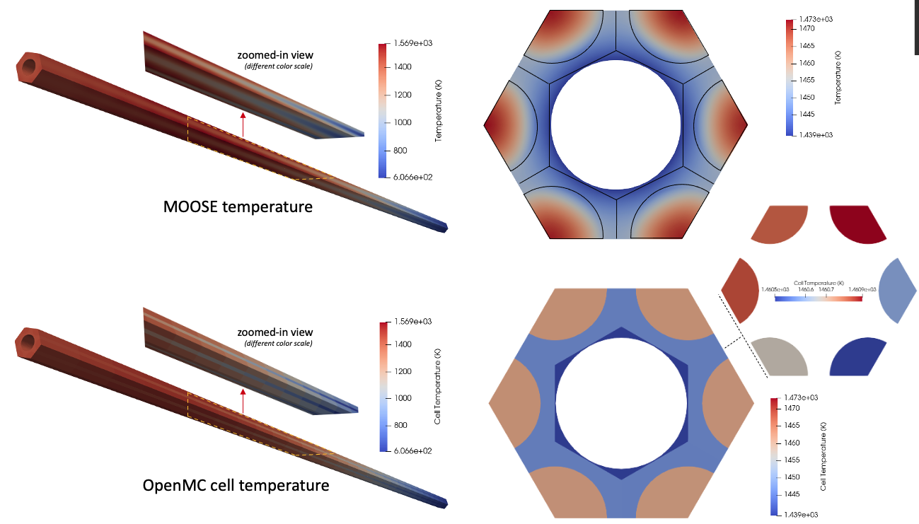
Figure 5: Temperature computed by MOOSE and applied to the OpenMC cells as volumes (left) and as slices at the top of the unit cell (right).
Figure 6 shows the fuel and graphite block temperatures as a function of axial position; each point is obtained by averaging over a slice parallel to the - plane. The graphite block temperature largely follows the imposed fluid temperature distribution, while the fuel compact temperature reaches a peak below the outlet because the fission power distribution is highest just slightly below the core mid-plane, as shown in Figure 4.
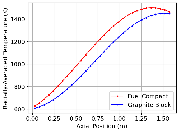
Figure 6: Radially-averaged fuel and graphite block temperatures in 30 axial layers
References
- INL.
High-Temperature Gas-Cooled Test Reactor Point Design.
Technical Report INL/EXT-16-38296, Idaho National Laboratory, 2016.
URL: https://tinyurl.com/v9a4hym5.[Export]
- A.J. Novak, D. Andrs, P. Shriwise, J. Fang, H. Yuan, D. Shaver, E. Merzari, P.K. Romano, and R.C. Martineau.
Coupled Monte Carlo and Thermal-Fluid Modeling of High Temperature Gas Reactors Using Cardinal.
Annals of Nuclear Energy, 177:109310, 2022.
doi:10.1016/j.anucene.2022.109310.[Export]
- A.J. Novak, R.W. Carlsen, S. Schunert, P. Balestra, D. Reger, R.N. Slaybaugh, and R.C. Martineau.
Pronghorn: A Multidimensional Coarse-Mesh Application for Advanced Reactor Thermal Hydraulics.
Nuclear Technology, 2021.[Export]
- H. Petersen.
The Properties of Helium: Density, Specific Heats, Viscosity, and Thermal Conductivity at Pressures from 1 to 100 bar and from Room Temperature to about 1800 K.
Technical Report, Danish Atomic Energy Commission, 1970.[Export]