Multiphysics for a TRISO Gas-Cooled Compact
In this tutorial, you will learn how to:
Couple OpenMC, NekRS/THM, and MOOSE together for multiphysics modeling of a TRISO compact
Use two different MultiApp hierarchies to achieve different data transfers
Use triggers to automatically terminate the OpenMC active batches once reaching the desired statistical uncertainty
Automatically detect steady state
To access this tutorial,
cd cardinal/tutorials/gas_compact_multiphysics
This tutorial also requires you to download mesh files and a NekRS restart file from Box. Please download the files from the gas_compact_multiphysics folder here and place these within the same directory structure in tutorials/gas_compact_multiphysics.
This tutorial requires HPC resources to run the NekRS cases. You will be able to run the OpenMC-THM-MOOSE files without any special resources.
In this tutorial, we couple OpenMC to the MOOSE heat transfer module, with fluid feedback provided by either NekRS or THM,
NekRS: wall-resolved - RANS equations
Thermal Hydraulics Module (THM): 1-D area-averaged Navier-Stokes equations
Two different multiapp hierarchies will be used in order to demonstrate the flexibility of the MultiApp system. The same OpenMC model can be used to provide feedback to different combinations of MOOSE applications.
In this tutorial, OpenMC receives temperature feedback from the MOOSE heat conduction module (for the solid regions) and NekRS/THM (for the fluid regions). Density feedback is provided by NekRS/THM for the fluid regions. This tutorial models a partial-height TRISO-fueled unit cell of a prismatic gas reactor assembly, and is a continuation of the conjugate heat transfer tutorial (where we coupled NekRS and MOOSE heat conduction) and the OpenMC-heat conduction tutorial (where we coupled OpenMC and MOOSE heat conduction) for this geometry.
This tutorial was developed with support from the NEAMS Thermal Fluids Center of Excellence and is described in more detail in our journal article Novak et al. (2022).
Geometry and Computational Model
The geometry consists of a TRISO-fueled gas reactor compact unit cell INL (2016). A top-down view of the geometry is shown in Figure 1. The fuel is cooled by helium flowing in a cylindrical channel of diameter . Cylindrical fuel compacts containing randomly-dispersed TRISO particles at 15% packing fraction are arranged around the coolant channel in a triangular lattice. The TRISO particles use a conventional design that consists of a central fissile uranium oxycarbide kernel enclosed in a carbon buffer, an inner PyC layer, a silicon carbide layer, and finally an outer PyC layer. The geometric specifications are summarized in Table 1. Heat is produced in the TRISO particles to yield a total power of 38 kW.
-fueled gas reactor compact unit cell](../media/compact_unit_cell.png)
Figure 1: TRISO-fueled gas reactor compact unit cell
Table 1: Geometric specifications for a TRISO-fueled gas reactor compact
| Parameter | Value (cm) |
|---|---|
| Coolant channel diameter, | 1.6 |
| Fuel compact diameter, | 1.27 |
| Fuel-to-coolant center distance, | 1.88 |
| Height | 160 |
| TRISO kernel radius | 214.85e-4 |
| Buffer layer radius | 314.85e-4 |
| Inner PyC layer radius | 354.85e-4 |
| Silicon carbide layer radius | 389.85e-4 |
| Outer PyC layer radius | 429.85e-4 |
Two different MultiApp hierarchies are used:
A "single stack" design where each application has either a single "parent" application or a single "child" application
A "tree" design where each application has a single "parent" application, but multiple "child" applications
Figure 2 shows a conceptual depiction of these hierarchies. We will describe these in greater detail later, but introduce them here to assist with describing a few aspects of the single-physics models. The circled numbers indicate the order in which the applications run.
Solid lines depict transfers that occur directly from application to application , or between the source and receiver of that field. Dashed lines, on the other hand, depict transfers that do not occur directly between the source and receiver of the field - for instance, in the "single stack" hierarchy, the NekRS application can only communicate data with it's immediate parent application. Therefore, to send fluid density and temperature from NekRS to OpenMC, there are actually two transfers - 1) sending fluid density and temperature from NekRS to the MOOSE heat transfer module, and 2) sending fluid density and temperature from the MOOSE heat transfer module to OpenMC.
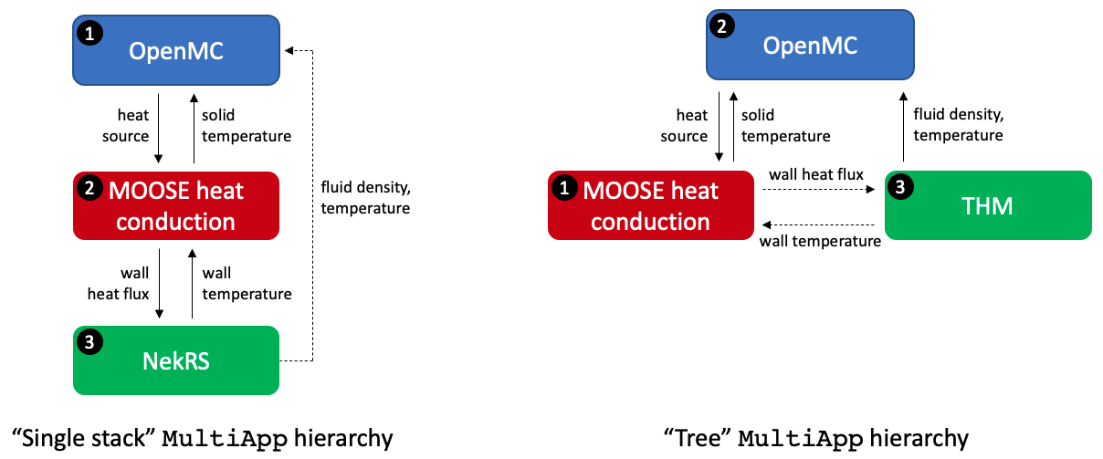
Figure 2: MultiApp hierarchies used in this tutorial; data transfers are shown with solid and dashed lines. Solid lines indicate transfers that occur directly from application A to application B, while dashed lines show transfers that have to first pass through an intermediate application to get to the eventual target application.
Conversely, with the "tree" hierarhcy, MOOSE MultiApps communicate with parent/child applications. Therefore, all data communicated between the MOOSE heat transfer module and THM actually has to first pass through their common parent application before reaching the desired target application.
In the time since we originally developed this tutorial, MOOSE has been extended to support sibling transfers, which would allow MOOSE and THM to communicate data directly to one another (in the "tree" hierarchy shown in Figure 2).
OpenMC Model
The OpenMC model is built using CSG. The TRISO positions are sampled using the Random Sequential Addition (RSA) algorithm in OpenMC. OpenMC's Python API is used to create the model with the script shown below. First, we define materials. Next, we create a single TRISO particle universe consisting of the five layers of the particle and an infinite extent of graphite filling all other space. We then pack pack uniform-radius spheres into a cylindrical region representing a fuel compact, setting each sphere to be filled with the TRISO universe.
#!/bin/env python

from argparse import ArgumentParser
import math
import numpy as np
import matplotlib.pyplot as plt

import openmc
import sys
import os

# Get common input parameters shared by other physics
script_dir = os.path.dirname(__file__)
sys.path.append(script_dir)
import common_input as specs
import materials as mats

def coolant_temp(t_in, t_out, l, z):
    """
    THIS IS ONLY USED FOR SETTING AN INITIAL CONDITION IN OPENMC's XML FILES -
    the coolant temperature will be applied from MOOSE, we just set an initial
    value here in case you want to run these files in standalone mode (i.e. with
    the "openmc" executable).

    Computes the coolant temperature based on an expected cosine power distribution
    for a specified temperature rise. The total core temperature rise is governed
    by energy conservation as dT = Q / m / Cp, where dT is the total core temperature
    rise, Q is the total core power, m is the mass flowrate, and Cp is the fluid
    isobaric specific heat. If you neglect axial heat conduction and assume steady
    state, then the temperature rise in a layer of fluid i can be related to the
    ratio of the power in that layer to the total power,
    dT_i / dT = Q_i / Q. We assume here a sinusoidal power distribution to get
    a reasonable estimate of an initial coolant temperature distribution.

    Parameters
    ----------

    t_in : float
        Inlet temperature of the channel
    t_out : float
        Outlet temperature of the channel
    l : float
        Length of the channel
    z : float or 1-D numpy.array
        Axial position where the temperature will be computed

    Returns
    -------
        float or 1-D numpy array of float depending on z
    """
    dT = t_out - t_in
    Q = 2 * l / math.pi
    distance_from_inlet = specs.unit_cell_height - z
    Qi = (l - l * np.cos(math.pi * distance_from_inlet / l)) / math.pi

    t = t_in + Qi / Q * dT

    return t

def coolant_density(t):
  """
    THIS IS ONLY USED FOR SETTING AN INITIAL CONDITION IN OPENMC's XML FILES -
    the coolant density will be applied from MOOSE, we just set an initial
    value here in case you want to run these files in standalone mode (i.e. with
    the "openmc" executable).

  Computes the helium density (kg/m3) from temperature assuming a fixed operating pressure.

  Parameters
  ----------

  t : float
    Fluid temperature

  Returns
  _______
    float or 1-D numpy array of float depending on t
  """

  p_in_bar = specs.outlet_P * 1.0e-5
  return 48.14 * p_in_bar / (t + 0.4446 * p_in_bar / math.pow(t, 0.2))

# -------------- Unit Conversions: OpenMC requires cm -----------
m = 100.0
# -------------------------------------------

### RADIANT UNIT CELL SPECS (INFERRED FROM REPORTS) ###

unit_cell_mdot = specs.mdot / (specs.n_bundles * specs.n_coolant_channels_per_block)
unit_cell_power = specs.power / (specs.n_bundles * specs.n_coolant_channels_per_block) * (specs.unit_cell_height / specs.height)

# estimate the outlet temperature using bulk energy conservation for steady state
coolant_outlet_temp = unit_cell_power / unit_cell_mdot / specs.fluid_Cp + specs.inlet_T

# geometry
coolant_channel_diam = specs.channel_diameter * m
reactor_bottom = 0.0
reactor_height = specs.unit_cell_height * m
reactor_top = reactor_bottom + reactor_height

### ARBITRARILY DETERMINED PARAMETERS ###

cell_pitch = specs.fuel_to_coolant_distance * m
fuel_channel_diam = specs.compact_diameter * m

hex_orientation = 'x'

def unit_cell(n_ax_zones, n_inactive, n_active):
    axial_section_height = reactor_height / n_ax_zones

    # superimposed search lattice
    triso_lattice_shape = (4, 4, int(axial_section_height))

    lattice_orientation = 'x'
    cell_edge_length = cell_pitch

    model = openmc.model.Model()

    ### Geometry ###

    # TRISO particle
    radius_pyc_outer       = specs.oPyC_radius * m

    s_fuel             = openmc.Sphere(r=specs.kernel_radius*m)
    s_c_buffer         = openmc.Sphere(r=specs.buffer_radius*m)
    s_pyc_inner        = openmc.Sphere(r=specs.iPyC_radius*m)
    s_sic              = openmc.Sphere(r=specs.SiC_radius*m)
    s_pyc_outer        = openmc.Sphere(r=radius_pyc_outer)
    c_triso_fuel       = openmc.Cell(name='c_triso_fuel'     , fill=mats.m_fuel,              region=-s_fuel)
    c_triso_c_buffer   = openmc.Cell(name='c_triso_c_buffer' , fill=mats.m_graphite_c_buffer, region=+s_fuel      & -s_c_buffer)
    c_triso_pyc_inner  = openmc.Cell(name='c_triso_pyc_inner', fill=mats.m_graphite_pyc,      region=+s_c_buffer  & -s_pyc_inner)
    c_triso_sic        = openmc.Cell(name='c_triso_sic'      , fill=mats.m_sic,               region=+s_pyc_inner & -s_sic)
    c_triso_pyc_outer  = openmc.Cell(name='c_triso_pyc_outer', fill=mats.m_graphite_pyc,      region=+s_sic       & -s_pyc_outer)
    c_triso_matrix     = openmc.Cell(name='c_triso_matrix'   , fill=mats.m_graphite_matrix,   region=+s_pyc_outer)
    u_triso            = openmc.Universe(cells=[c_triso_fuel, c_triso_c_buffer, c_triso_pyc_inner, c_triso_sic, c_triso_pyc_outer, c_triso_matrix])

    # Channel surfaces
    fuel_cyl = openmc.ZCylinder(r=0.5 * fuel_channel_diam)
    coolant_cyl = openmc.ZCylinder(r=0.5 * coolant_channel_diam)

    # create a TRISO lattice for one axial section (to be used in the rest of the axial zones)
    # center the TRISO region on the origin so it fills lattice cells appropriately
    min_z = openmc.ZPlane(z0=-0.5 * axial_section_height)
    max_z = openmc.ZPlane(z0=0.5 * axial_section_height)

    # region in which TRISOs are generated
    r_triso = -fuel_cyl & +min_z & -max_z

    rand_spheres = openmc.model.pack_spheres(radius=radius_pyc_outer, region=r_triso, pf=specs.triso_pf, seed=1.0)
    random_trisos = [openmc.model.TRISO(radius_pyc_outer, u_triso, i) for i in rand_spheres]

    llc, urc = r_triso.bounding_box
    pitch = (urc - llc) / triso_lattice_shape
    # insert TRISOs into a lattice to accelerate point location queries
    triso_lattice = openmc.model.create_triso_lattice(random_trisos, llc, pitch, triso_lattice_shape, mats.m_graphite_matrix)

    # create a hexagonal lattice for the coolant and fuel channels
    fuel_univ = openmc.Universe(cells=[openmc.Cell(region=-fuel_cyl, fill=triso_lattice),
                                    openmc.Cell(region=+fuel_cyl, fill=mats.m_graphite_matrix)])

    # extract the coolant cell and set temperatures based on the axial profile
    coolant_cell = openmc.Cell(region=-coolant_cyl, fill=mats.m_coolant)
    # set the coolant temperature on the cell to approximately match the expected
    # temperature profile
    axial_coords = np.linspace(reactor_bottom, reactor_top, n_ax_zones + 1)
    lattice_univs = []

    fuel_ch_cells = []

    i = 0
    for z_min, z_max in zip(axial_coords[0:-1], axial_coords[1:]):
        # create a new coolant universe for each axial zone in the coolant channel;
        # this generates a new material as well (we only need to do this for all
        # cells except the first cell)
        if (i == 0):
          c_cell = coolant_cell
        else:
          c_cell = coolant_cell.clone(clone_materials = False)

        i += 1

        # use the middle of the axial section to compute the temperature and density
        ax_pos = 0.5 * (z_min + z_max)
        t = coolant_temp(specs.inlet_T, coolant_outlet_temp, reactor_height, ax_pos)

        # Set the temperature in Kelvin
        c_cell.temperature = t
        # Set the density in g/cc
        c_cell.density = coolant_density(t) / 1000.0

        # set the solid cells and their temperatures
        graphite_cell = openmc.Cell(region=+coolant_cyl, fill=mats.m_graphite_matrix)
        fuel_ch_cell = openmc.Cell(region=-fuel_cyl, fill=triso_lattice)
        fuel_ch_matrix_cell = openmc.Cell(region=+fuel_cyl, fill=mats.m_graphite_matrix)

        graphite_cell.temperature = t
        fuel_ch_cell.temperature = t
        fuel_ch_matrix_cell.temperature = t

        fuel_ch_cells.append(fuel_ch_cell)
        fuel_u = openmc.Universe(cells=[fuel_ch_cell, fuel_ch_matrix_cell])
        coolant_u = openmc.Universe(cells=[c_cell, graphite_cell])
        lattice_univs.append([[fuel_u] * 6, [coolant_u]])

    # create a hexagonal lattice used in each axial zone to represent the cell
    hex_lattice = openmc.HexLattice(name="Unit cell lattice")
    hex_lattice.orientation = lattice_orientation
    hex_lattice.center = (0.0, 0.0, 0.5 * (reactor_bottom + reactor_top))
    hex_lattice.pitch = (cell_pitch, axial_section_height)
    hex_lattice.universes = lattice_univs

    graphite_outer_cell = openmc.Cell(fill=mats.m_graphite_matrix)
    graphite_outer_cell.temperature = t
    inf_graphite_univ = openmc.Universe(cells=[graphite_outer_cell])
    hex_lattice.outer = inf_graphite_univ

    # hexagonal bounding cell
    hex = openmc.model.HexagonalPrism(cell_edge_length, hex_orientation, boundary_type='periodic')

    hex_cell_vol = 6.0 * (math.sqrt(3) / 4.0) * cell_edge_length**2 * reactor_height

    # create additional axial regions
    axial_planes = [openmc.ZPlane(z0=coord) for coord in axial_coords]
    # axial planes
    min_z = axial_planes[0]
    min_z.boundary_type = 'vacuum'
    max_z = axial_planes[-1]
    max_z.boundary_type = 'vacuum'

    # fill the unit cell with the hex lattice
    hex_cell = openmc.Cell(region=-hex & +min_z & -max_z, fill=hex_lattice)

    model.geometry = openmc.Geometry([hex_cell])

    ### Settings ###
    settings = openmc.Settings()

    settings.particles = 150000
    settings.inactive = n_inactive
    settings.batches = settings.inactive + n_active

    # the only reason we use 'nearest' here is to be sure we have a robust test for CI;
    # otherwise, 1e-16 differences in temperature (due to numerical roundoff when using
    # different MPI ranks) do change the tracking do to the stochastic interpolation
    settings.temperature['method'] = 'nearest'
    settings.temperature['range'] = (294.0, 1500.0)
    settings.temperature['tolerance'] = 200.0

    hexagon_half_flat = math.sqrt(3.0) / 2.0 * cell_edge_length
    lower_left = (-cell_edge_length, -hexagon_half_flat, reactor_bottom)
    upper_right = (cell_edge_length, hexagon_half_flat, reactor_top)
    source_dist = openmc.stats.Box(lower_left, upper_right)
    source = openmc.IndependentSource(space=source_dist)
    settings.source = source

    model.settings = settings

    m_colors = {}
    m_colors[mats.m_coolant] = 'royalblue'
    m_colors[mats.m_fuel] = 'red'
    m_colors[mats.m_graphite_c_buffer] = 'black'
    m_colors[mats.m_graphite_pyc] = 'orange'
    m_colors[mats.m_sic] = 'yellow'
    m_colors[mats.m_graphite_matrix] = 'silver'

    plot1          = openmc.Plot()
    plot1.filename = 'plot1'
    plot1.width    = (2 * cell_pitch, 4 * axial_section_height)
    plot1.basis    = 'xz'
    plot1.origin   = (0.0, 0.0, reactor_height/2.0)
    plot1.pixels   = (int(800 * 2 * cell_pitch), int(800 * 4 * axial_section_height))
    plot1.color_by = 'cell'

    plot2          = openmc.Plot()
    plot2.filename = 'plot2'
    plot2.width    = (3 * cell_pitch, 3 * cell_pitch)
    plot2.basis    = 'xy'
    plot2.origin   = (0.0, 0.0, axial_section_height / 2.0)
    plot2.pixels   = (int(800 * cell_pitch), int(800 * cell_pitch))
    plot2.color_by = 'material'
    plot2.colors   = m_colors

    plot3          = openmc.Plot()
    plot3.filename = 'plot3'
    plot3.width    = plot2.width
    plot3.basis    = plot2.basis
    plot3.origin   = plot2.origin
    plot3.pixels   = plot2.pixels
    plot3.color_by = 'cell'

    model.plots = openmc.Plots([plot1, plot2, plot3])

    return model

def main():

    ap = ArgumentParser()
    ap.add_argument('-n', dest='n_axial', type=int, default=50,
                    help='Number of axial cell divisions')
    ap.add_argument('-i', dest='n_inactive', type=int, default=20,
                    help='Number of inactive cycles')
    ap.add_argument('-a', dest='n_active', type=int, default=45,
                    help='Number of active cycles')

    args = ap.parse_args()

    model = unit_cell(args.n_axial, args.n_inactive, args.n_active)
    model.export_to_xml()

if __name__ == "__main__":
    main()
Finally, we loop over axial layers and create unique cells for each of the six compacts, the graphite block, and the coolant. Recall that we need unique cells in order for each region to obtain a a unique temperature from MOOSE. The level on which we will apply feedback from MOOSE is set to 1 because each layer is a component in a lattice nested once with respect to the highest level. To accelerate the particle tracking, we:
Repeat the same TRISO universe in each axial layer and within each compact
Superimpose a Cartesian search lattice in the fuel channel regions.
The OpenMC geometry, colored by cell ID, is shown in Figure 3. The lateral faces of the unit cell are periodic, while the top and bottom boundaries are vacuum. The Cartesian search lattice in the fuel compact regions is also visible.
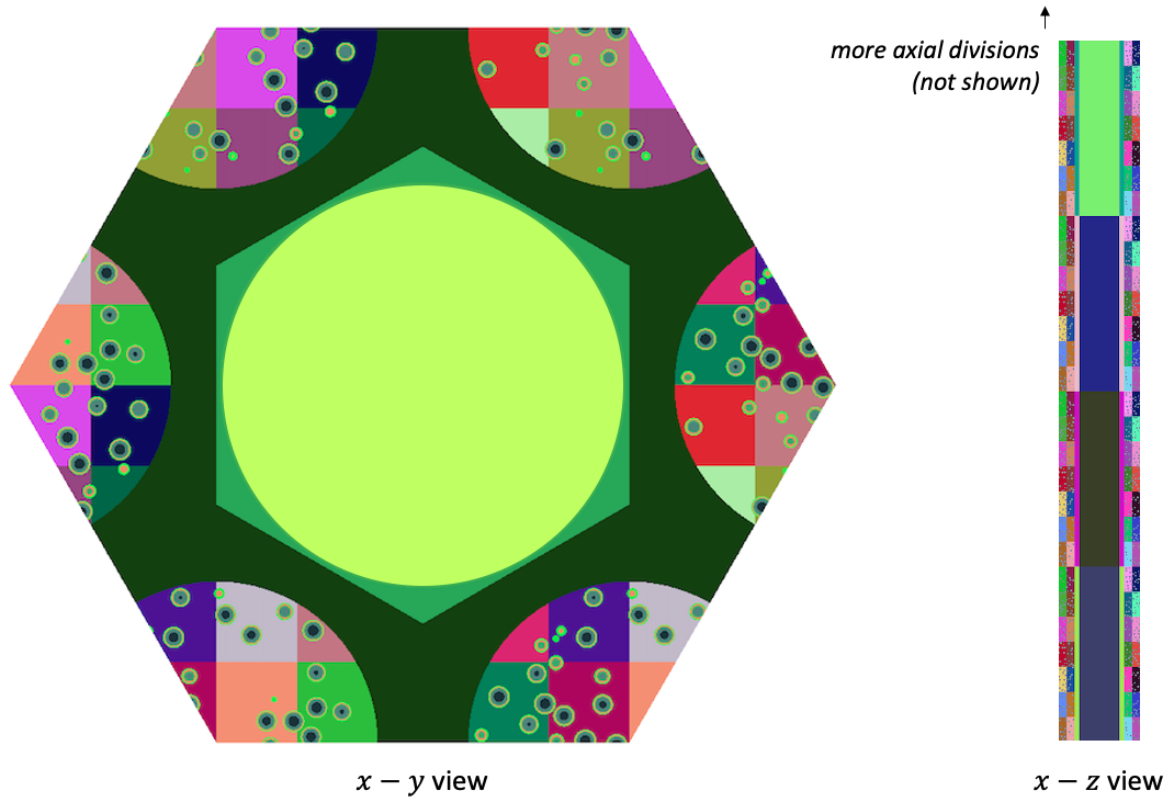
Figure 3: OpenMC model, colored by cell ID
For the "single-stack" MultiApp hierarchy, OpenMC runs first, so the initial temperature is set to uniform in the radial direction and given by a linear variation between the inlet and outlet fluid temperatures. The fluid density is then set using the ideal gas EOS with pressure taken as the fixed outlet of 7.1 MPa given the temperature, i.e. . For the "tree" MultiApp hierarchy, OpenMC instead runs after the MOOSE heat transfer module, but before THM. For this structure, initial conditions are only required for fluid temperature and density, which are taken as the same initial conditions as for the "single-stack" case.
To create the XML files required to run OpenMC, run the script:
python unit_cell.py
You can also use the XML files checked in to the tutorials/gas_compact_multiphysics directory.
Heat Conduction Model
The MOOSE heat transfer module is used to solve for energy conservation in the solid. The solid mesh is shown in Figure 4; the only sideset defined in the domain is the coolant channel surface. The solid geometry uses a length unit of meters.
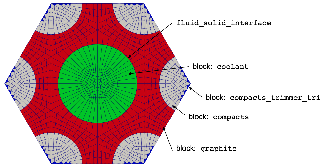
Figure 4: Mesh for the solid heat conduction model
This mesh is generated using MOOSE mesh generators in the solid_mesh.i file.
[Mesh<<<{"href": "../syntax/Mesh/index.html"}>>>]
  [fuel_pin]
    type = PolygonConcentricCircleMeshGenerator<<<{"description": "This PolygonConcentricCircleMeshGenerator object is designed to mesh a polygon geometry with optional rings centered inside.", "href": "../source/meshgenerators/PolygonConcentricCircleMeshGenerator.html"}>>>
    num_sides<<<{"description": "Number of sides of the polygon."}>>> = 6
    polygon_size<<<{"description": "Size of the polygon to be generated (given as either apothem or radius depending on polygon_size_style)."}>>> = '${fparse fuel_to_coolant_distance / 2.0}'
    ring_radii<<<{"description": "Radii of major concentric circles (rings)."}>>> = '${fparse 0.8 * compact_diameter / 2.0} ${fparse compact_diameter / 2.0}'
    ring_intervals<<<{"description": "Number of radial mesh intervals within each major concentric circle excluding their boundary layers."}>>> = '1 1'
    num_sectors_per_side<<<{"description": "Number of azimuthal sectors per polygon side (rotating counterclockwise from top right face)."}>>> = '${ns} ${ns} ${ns} ${ns} ${ns} ${ns}'
    ring_block_ids<<<{"description": "Optional customized block ids for each ring geometry block."}>>> = '2 2'
    ring_block_names<<<{"description": "Optional customized block names for each ring geometry block."}>>> = 'compacts compacts'
    background_block_names<<<{"description": "Optional customized block names for the background block."}>>> = 'graphite'
    background_intervals<<<{"description": "Number of radial meshing intervals in background region (area between rings and ducts) excluding the background's boundary layers."}>>> = 4
  []
  [coolant_pin]
    type = PolygonConcentricCircleMeshGenerator<<<{"description": "This PolygonConcentricCircleMeshGenerator object is designed to mesh a polygon geometry with optional rings centered inside.", "href": "../source/meshgenerators/PolygonConcentricCircleMeshGenerator.html"}>>>
    num_sides<<<{"description": "Number of sides of the polygon."}>>> = 6
    polygon_size<<<{"description": "Size of the polygon to be generated (given as either apothem or radius depending on polygon_size_style)."}>>> = '${fparse fuel_to_coolant_distance / 2.0}'
    ring_radii<<<{"description": "Radii of major concentric circles (rings)."}>>> = '${fparse channel_diameter / 2.0}'
    ring_intervals<<<{"description": "Number of radial mesh intervals within each major concentric circle excluding their boundary layers."}>>> = '2'
    num_sectors_per_side<<<{"description": "Number of azimuthal sectors per polygon side (rotating counterclockwise from top right face)."}>>> = '${ns} ${ns} ${ns} ${ns} ${ns} ${ns}'
    ring_block_ids<<<{"description": "Optional customized block ids for each ring geometry block."}>>> = '101 101'
    ring_block_names<<<{"description": "Optional customized block names for each ring geometry block."}>>> = 'coolant coolant'
    background_block_names<<<{"description": "Optional customized block names for the background block."}>>> = 'graphite'
    interface_boundary_id_shift<<<{"description": "Integer used to shift interface boundary IDs."}>>> = 100
    background_intervals<<<{"description": "Number of radial meshing intervals in background region (area between rings and ducts) excluding the background's boundary layers."}>>> = 3
  []
  [bundle]
    type = PatternedHexMeshGenerator<<<{"description": "This PatternedHexMeshGenerator source code assembles hexagonal meshes into a hexagonal grid and optionally forces the outer boundary to be hexagonal and/or adds a duct.", "href": "../source/meshgenerators/PatternedHexMeshGenerator.html"}>>>
    inputs<<<{"description": "The input MeshGenerators."}>>> = 'fuel_pin coolant_pin'
    hexagon_size<<<{"description": "Size of the outmost hexagon boundary to be generated; this is required only when pattern type is 'hexagon'."}>>> = '${fparse 2.0 * fuel_to_coolant_distance}'
    pattern<<<{"description": "A double-indexed hexagonal-shaped array starting with the upper-left corner."}>>> = '0 0;
              0 1 0;
               0 0'
  []
  [trim]
    type = HexagonMeshTrimmer<<<{"description": "This HexagonMeshTrimmer object performs peripheral and/or across-center (0, 0, 0) trimming for assembly or core 2D meshes generated by PatternedHexMG.", "href": "../source/meshgenerators/HexagonMeshTrimmer.html"}>>>
    input<<<{"description": "The input mesh that needs to be trimmed."}>>> = bundle
    trim_peripheral_region<<<{"description": "Whether the peripheral region on each of the six sides will be trimmed in an assembly mesh. See documentation for numbering convention."}>>> = '1 1 1 1 1 1'
    peripheral_trimming_section_boundary<<<{"description": "Boundary formed by peripheral trimming."}>>> = peripheral_section
  []
  [rotate]
    type = TransformGenerator<<<{"description": "Applies a linear transform to the entire mesh.", "href": "../source/meshgenerators/TransformGenerator.html"}>>>
    input<<<{"description": "The mesh we want to modify"}>>> = trim
    transform<<<{"description": "The type of transformation to perform (TRANSLATE, TRANSLATE_CENTER_ORIGIN, TRANSLATE_MIN_ORIGIN, ROTATE, SCALE, ROTATE_WITH_MATRIX, ROTATE_EXT)"}>>> = rotate
    vector_value<<<{"description": "The value to use for the transformation. When using TRANSLATE or SCALE, the xyz coordinates are applied in each direction respectively. When using ROTATE, the values are interpreted as the Euler angles phi, theta and psi given in degrees. For ROTATE_EXT, an extrinsic rotation is carried out using prescribed Euler angles alpha, beta, and gamma in degrees."}>>> = '30.0 0.0 0.0'
  []
  [extrude]
    type = AdvancedExtruderGenerator<<<{"description": "Extrudes a 1D mesh into 2D, or a 2D mesh into 3D, and supports a variable height for each elevation, variable number of layers within each elevation, variable growth factors of axial element sizes within each elevation and remap subdomain_ids, boundary_ids and element extra integers within each elevation as well as interface boundaries between neighboring elevation layers, as well as following a 1D curve and modifying the radial (normal to the extrusion axis) extent of the geometry.", "href": "../source/meshgenerators/AdvancedExtruderGenerator.html"}>>>
    input<<<{"description": "The mesh to extrude"}>>> = rotate
    heights<<<{"description": "The height of each elevation"}>>> = ${height}
    num_layers<<<{"description": "The number of layers for each elevation - must be num_elevations in length!"}>>> = ${n_layers}
    direction<<<{"description": "A vector that points in the direction to extrude (note, this will be normalized internally - so don't worry about it here)"}>>> = '0 0 1'
  []
  [fluid_solid_interface]
    type = SideSetsBetweenSubdomainsGenerator<<<{"description": "MeshGenerator that creates a sideset composed of the nodes located between two or more subdomains.", "href": "../source/meshgenerators/SideSetsBetweenSubdomainsGenerator.html"}>>>
    input<<<{"description": "The mesh we want to modify"}>>> = extrude
    primary_block<<<{"description": "The primary set of blocks for which to draw a sideset between"}>>> = 'graphite'
    paired_block<<<{"description": "The paired set of blocks for which to draw a sideset between"}>>> = 'coolant'
    new_boundary<<<{"description": "The list of boundary names to create on the supplied subdomain"}>>> = 'fluid_solid_interface'
  []
[]We first create a full 7-pin bundle, and then apply a trimming operation to split the compacts. Because MOOSE does not support multiple element types (e.g. tets, hexes) on the same block ID, the trimmer automatically creates an additional block (compacts_trimmer_tri) to represent the triangular prism elements formed in the compacts. Note that within this mesh, we include the fluid region - for the "single stack" MultiApp hierarchy, we will need somewhere for NekRS to write the fluid temperature solution. So, while this block does not participate in the solid solve, we include it in the mesh just for data transfers. You can generate this mesh by running
cardinal-opt -i solid_mesh.i --mesh-only
which will create the mesh, named solid_mesh_in.e.
On the coolant channel surface, a Dirichlet temperature is provided by NekRS/THM. All other boundaries are insulated. The volumetric power density is provided by OpenMC, with normalization to ensure the total specified power. When using the "single stack" hierarchy, MOOSE runs after OpenMC but before NekRS, and an initial condition is only required for the wall temperature, which is set to a linear variation from inlet to outlet fluid temperature. When using the "tree" hierarchy, MOOSE runs first, in which case the initial wall temperature is taken as the same linear variation, while the power is taken as uniform.
NekRS Model
NekRS is used to solve the incompressible k-tau RANS model. The inlet mass flowrate is 0.0905 kg/s; with the channel diameter of 1.6 cm and material properties of helium, this results in a Reynolds number of 223214 and a Prandtl number of 0.655. This highly-turbulent flow results in extremely thin momentum and thermal boundary layers on the no-slip surfaces forming the periphery of the coolant channel. In order to resolve the near-wall behavior with a wall-resolved model, an extremely fine mesh is required in the NekRS simulation. To accelerate the overall coupled solve that is of interest in this tutorial, the NekRS model is split into a series of calculations:
We first run a partial-height, periodic flow-only case to obtain converged , , and distributions.
Then, we extrapolate the and to the full-height case.
We use the converged, full-height and distributions to transport a temperature passive scalar in a CHT calculation with MOOSE.
Finally, we use the converged CHT case as an initial condition for the multiphysics simulation with OpenMC and MOOSE feedback.
Steps 1-3 were performed in an earlier tutorial - for brevity, we skip repeating the discussion of steps 1-3.
For the multiphysics case, we will load the restart file produced from step 3, compute from the loaded solutions for and , and then transport temperature with coupling to MOOSE heat conduction and OpenMC particle transport. Let's now describe the NekRS input files needed for the passive scalar solve:
ranstube.re2: NekRS meshranstube.par: High-level settings for the solver, boundary condition mappings to sidesets, and the equations to solveranstube.udf: User-defined C++ functions for on-line postprocessing and model setupranstube.oudf: User-defined OCCA kernels for boundary conditions and source terms
A detailed description of all of the available parameters, settings, and use cases for these input files is available on the NekRS documentation website. Because the purpose of this analysis is to demonstrate Cardinal's capabilities, only the aspects of NekRS required to understand the present case will be covered. First, the NekRS mesh is shown in Figure 5. Boundary 1 is the inlet, boundary 2 is the outlet, and boundary 3 is the wall. The same mesh was used for the periodic flow solve, except with a shorter height.
 model](../media/nek_mesh_uc.png)
Figure 5: Mesh for the NekRS RANS model
Next, the .par file contains problem setup information. This input sets up a nondimensional passive scalar solution, loading , , , and from a restart file. We "freeze" the flow by setting solver = none in the [VELOCITY], [SCALAR01] ( passive scalar), and [SCALAR02] ( passive scalar) blocks. In the nondimensional formulation, the "viscosity" becomes , where is the Reynolds number, while the "thermal conductivity" becomes , where is the Peclet number. These nondimensional numbers are used to set various diffusion coefficients in the governing equations with syntax like -223214, which is equivalent in NekRS syntax to . The only equation that NekRS will solve is for temperature.
# Model of a turbulent channel flow.
#
# L_ref = 0.016 m          coolant channel diameter
# T_ref = 598 K            coolant inlet temperature
# dT_ref = 82.89 K         coolant nominal temperature rise in the unit cell
# U_ref = 81.089           coolant inlet velocity
# length = 1.6 m           coolant channel flow length
#
# rho_0 = 5.5508 kg/m3     coolant density
# mu_0 = 3.22639e-5 Pa-s   coolant dynamic viscosity
# Cp_0 = 5189 J/kg/K       coolant isobaric heat capacity
# k_0 = 0.2556 W/m/K       coolant thermal conductivity
#
# Re = 223214
# Pr = 0.655
# Pe = 146205

[GENERAL]
  startFrom = converged_cht.fld

  polynomialOrder = 7
  dt = 6e-3
  timeStepper = BDF2

  # end the simulation at specified number of time steps
  stopAt = numSteps
  numSteps = 1000

  # write an output file every specified time steps
  writeControl = steps
  writeInterval = 1000

[PROBLEMTYPE]
  stressFormulation = true

[PRESSURE]
  residualTol = 1e-04

[VELOCITY]
  solver = none
  viscosity = -223214
  density = 1.0
  boundaryTypeMap = v, o, W
  residualTol = 1e-06

[TEMPERATURE]
  rhoCp = 1.0
  conductivity = -146205
  boundaryTypeMap = t, o, f
  residualTol = 1e-06

[SCALAR01] # k
  solver = none
  boundaryTypeMap = t, I, o
  residualTol = 1e-06
  rho = 1.0
  diffusivity = -223214

[SCALAR02] # tau
  solver = none
  boundaryTypeMap = t, I, o
  residualTol = 1e-06
  rho = 1.0
  diffusivity = -223214
Next, the .udf file is used to setup initial conditions and define how should be computed based on and the restart values of and . In turbulent_props, a user-defined function, we use from the input file in combination with the and (read from the restart file later in the .udf file) to adjust the total diffusion coefficient on temperature to according to the turbulent Prandtl number definition. This adjustment must happen on device, in a new GPU kernel we name scalarScaledAddKernel. This kernel will be defined in the .oudf file; we instruct the JIT compilation to compile this new kernel by calling udfBuildKernel.
Then, in UDF_Setup we store the value of computed in the restart file.
#include <math.h>
#include "udf.hpp"

occa::memory o_mu_t_from_restart;

#define length 100.0    // non-dimensional channel length
#define Pr_T 0.91       // turbulent Prandtl number

static occa::kernel scalarScaledAddKernel;

void turbulent_props(nrs_t *nrs, double time, occa::memory o_U, occa::memory o_S,
            occa::memory o_UProp, occa::memory o_SProp)
{
  // fetch the laminar thermal conductivity and specify the desired turbulent Pr
  dfloat k_laminar;
  platform->options.getArgs("SCALAR00 DIFFUSIVITY", k_laminar);

  // o_diff is the turbulent conductivity for all passive scalars, so we grab the first
  // slice, since temperature is the first passive scalar
  occa::memory o_mu = nrs->cds->o_diff + 0 * nrs->cds->fieldOffset[0] * sizeof(dfloat);

  scalarScaledAddKernel(0, nrs->cds->mesh[0]->Nlocal, k_laminar, 1.0 / Pr_T,
    o_mu_t_from_restart /* turbulent viscosity */, o_mu /* laminar viscosity */);
}

void UDF_LoadKernels(occa::properties & kernelInfo)
{
  scalarScaledAddKernel = oudfBuildKernel(kernelInfo, "scalarScaledAdd");
}

void UDF_Setup(nrs_t *nrs)
{
  mesh_t *mesh = nrs->cds->mesh[0];
  int n_gll_points = mesh->Np * mesh->Nelements;

  // allocate space for the k and tau that we will read from the file
  dfloat * mu_t = (dfloat *) calloc(n_gll_points, sizeof(dfloat));

  for (int n = 0; n < n_gll_points; ++n)
  {
    // fetch the restart value of mu_T, which is equal to k * tau, the second and third
    // passive scalars
    mu_t[n] = nrs->cds->S[n + 1 * nrs->cds->fieldOffset[0]] *
              nrs->cds->S[n + 2 * nrs->cds->fieldOffset[0]];
  }

  o_mu_t_from_restart = platform->device.malloc(n_gll_points * sizeof(dfloat), mu_t);

  udf.properties = &turbulent_props;
}

void UDF_ExecuteStep(nrs_t * nrs, double time, int tstep)
{
}
In the .oudf file, we define boundary conditions for temperature and also the form of the scalarScaledAdd kernel that we use to compute . The inlet boundary is set to a temperature of 0 (a dimensional temperature of ), while the fluid-solid interface will receive a heat flux from MOOSE.
@kernel void scalarScaledAdd(const dlong offset, const dlong N,
                             const dfloat a,
                             const dfloat b,
                             @restrict const dfloat* X,
                             @restrict dfloat* Y)
{
  for (dlong n = 0; n < N; ++n; @tile(256,@outer,@inner))
    if (n < N)
      Y[n] = a + b * X[n + offset];
}

// Boundary conditions are only needed for temperature, since the solves of pressure,
// velocity, k, and tau are all frozen

void scalarDirichletConditions(bcData *bc)
{
  // inlet temperature
  bc->s = 0.0;
}

void scalarNeumannConditions(bcData *bc)
{
  // wall temperature
  // note: when running with Cardinal, Cardinal will allocate the usrwrk
  // array. If running with NekRS standalone (e.g. nrsmpi), you need to
  // replace the usrwrk with some other value or allocate it youself from
  // the udf and populate it with values.
  bc->flux = bc->usrwrk[bc->idM];
}
For this tutorial, NekRS runs last in the "single-stack" MultiApp hierarchy, so no initial conditions are required aside from the , , and taken from the converged_cht.fld restart file on Box.
THM Model
THM is used to solve the 1-D area-averaged Navier-Stokes equations. The THM mesh contains 150 elements; the mesh is constucted automatically within THM. The fluid geometry uses a length unit of meters. The heat flux imposed in the THM elements is obtained by area averaging the heat flux from the heat conduction model in 150 layers along the fluid-solid interface. For the reverse transfer, the wall temperature sent to MOOSE heat conduction is set to a uniform value along the fluid-solid interface according to a nearest-node mapping to the THM elements.
For this tutorial, THM runs last in the "tree" MultiApp hierarchy; because THM solves time-dependent equations, initial conditions are only required for the solution variables for which THM solves - pressure, fluid temperature, and velocity, all of which are set to uniform conditions.
Multiphysics Coupling
In this section, OpenMC, NekRS/THM, and MOOSE heat conduction are coupled for multiphysics modeling of the TRISO gas compact. Two separate simulations are performed here:
Coupling of OpenMC, NekRS, and MOOSE heat conduction in a "single-stack" MultiApp hierarchy
Coupling of OpenMC, THM, and MOOSE heat conduction in a "tree" MultiApp hierarchy
By individually describing the two setups, you will understand the customizability of the MultiApp system and the flexibility shared by all MOOSE applications for seamlessly exchanging tools of varying resolution for one another.
OpenMC-NekRS-MOOSE
In this section, we describe the coupling of OpenMC, NekRS, and MOOSE in the "single-stack" MultiApp hierarchy shown in Figure 2.
OpenMC Input Files
The neutronics physics is solved over the entire domain with OpenMC. The OpenMC wrapping used for the OpenMC-NekRS-MOOSE coupling is described in the openmc_nek.i input file. We begin by defining a number of constants and by setting up the mesh mirror on which OpenMC will receive temperature and density from THM-MOOSE, and on which OpenMC will write the fission heat source. Because the coupled applications use length units of meters, the mesh mirror must also be in units of meters. For simplicity, we just use the same mesh as generated with solid_mesh.i earlier, though this it not necessary.
!include common_input.i

# This input file runs coupled OpenMC Monte Carlo transport, MOOSE heat
# conduction, and NekRS fluid flow and heat transfer.
# This input should be run with:
#
# cardinal-opt -i openmc_nek.i

num_layers_for_THM = 150
density_blocks = 'coolant'
temperature_blocks = 'graphite compacts compacts_trimmer_tri'
fuel_blocks = 'compacts compacts_trimmer_tri'

unit_cell_power = ${fparse power / (n_bundles * n_coolant_channels_per_block) * unit_cell_height / height}

U_ref = ${fparse mdot / (n_bundles * n_coolant_channels_per_block) / fluid_density / (pi * channel_diameter * channel_diameter / 4.0)}
t0 = ${fparse channel_diameter / U_ref}
nek_dt = 6e-3
N = 1000

[Mesh]
  [solid]
    type = FileMeshGenerator
    file = solid_mesh_in.e
  []
[]
Next, we define a number of auxiliary variables to query the OpenMC solution and set up multiphysics coupling. We add cell_temperature and cell_density in order to read the cell temperatures and densities directly from OpenMC in order to visualize the temperatures and densities ultimately applied to OpenMC's cells. In order to compute density using the ideal gas EOS given a temperature and a fixed pressure, we use a FluidDensityAux to set density.
[AuxVariables<<<{"href": "../syntax/AuxVariables/index.html"}>>>]
  [cell_temperature]
    family<<<{"description": "Specifies the family of FE shape functions to use for this variable"}>>> = MONOMIAL
    order<<<{"description": "Specifies the order of the FE shape function to use for this variable (additional orders not listed are allowed)"}>>> = CONSTANT
  []
  [cell_density]
    family<<<{"description": "Specifies the family of FE shape functions to use for this variable"}>>> = MONOMIAL
    order<<<{"description": "Specifies the order of the FE shape function to use for this variable (additional orders not listed are allowed)"}>>> = CONSTANT
  []
[]

[AuxKernels<<<{"href": "../syntax/AuxKernels/index.html"}>>>]
  [cell_temperature]
    type = CellTemperatureAux<<<{"description": "OpenMC cell temperature (K), mapped to each MOOSE element", "href": "../source/auxkernels/CellTemperatureAux.html"}>>>
    variable<<<{"description": "The name of the variable that this object applies to"}>>> = cell_temperature
  []
  [cell_density]
    type = CellDensityAux<<<{"description": "OpenMC fluid density (kg/m$^3$), mapped to each MOOSE element", "href": "../source/auxkernels/CellDensityAux.html"}>>>
    variable<<<{"description": "The name of the variable that this object applies to"}>>> = cell_density
  []
  [density]
    type = FluidDensityAux<<<{"description": "Computes density from pressure and temperature", "href": "../source/auxkernels/FluidDensityAux.html"}>>>
    variable<<<{"description": "The name of the variable that this object applies to"}>>> = density
    p<<<{"description": "Pressure"}>>> = ${outlet_P}
    T<<<{"description": "Temperature"}>>> = nek_temp
    fp<<<{"description": "The name of the user object for fluid properties"}>>> = helium
    execute_on<<<{"description": "The list of flag(s) indicating when this object should be executed. For a description of each flag, see https://mooseframework.inl.gov/source/interfaces/SetupInterface.html."}>>> = 'timestep_begin'
  []
[]

[FluidProperties<<<{"href": "../syntax/FluidProperties/index.html"}>>>]
  [helium]
    type = IdealGasFluidProperties<<<{"description": "Fluid properties for an ideal gas", "href": "../source/fluidproperties/IdealGasFluidProperties.html"}>>>
    molar_mass<<<{"description": "Constant molar mass of the fluid (kg/mol)"}>>> = 4e-3
    gamma<<<{"description": "gamma value (cp/cv)"}>>> = 1.668282 # should correspond to  Cp = 5189 J/kg/K
    k<<<{"description": "Thermal conductivity, W/(m-K)"}>>> = 0.2556
    mu<<<{"description": "Dynamic viscosity, Pa.s"}>>> = 3.22639e-5
  []
[]Next, we define the necessary initial conditions using functions; all temperatures (nek_temp and solid_temp are to be discussed shortly) are set to a linear variation from the inlet to outlet fluid temperatures.
[ICs<<<{"href": "../syntax/Cardinal/ICs/index.html"}>>>]
  [temp]
    type = FunctionIC<<<{"description": "An initial condition that uses a normal function of x, y, z to produce values (and optionally gradients) for a field variable.", "href": "../source/ics/FunctionIC.html"}>>>
    variable<<<{"description": "The variable this initial condition is supposed to provide values for."}>>> = nek_temp
    function<<<{"description": "The initial condition function."}>>> = temp_ic
  []
  [solid_temp]
    type = FunctionIC<<<{"description": "An initial condition that uses a normal function of x, y, z to produce values (and optionally gradients) for a field variable.", "href": "../source/ics/FunctionIC.html"}>>>
    variable<<<{"description": "The variable this initial condition is supposed to provide values for."}>>> = solid_temp
    function<<<{"description": "The initial condition function."}>>> = temp_ic
  []
[]

[Functions<<<{"href": "../syntax/Functions/index.html"}>>>]
  [temp_ic]
    type = ParsedFunction<<<{"description": "Function created by parsing a string", "href": "../source/functions/MooseParsedFunction.html"}>>>
    expression<<<{"description": "The user defined function."}>>> = '${inlet_T} + z / ${unit_cell_height} * ${unit_cell_power} / (${mdot} / ${n_bundles} / ${n_coolant_channels_per_block}) / ${fluid_Cp}'
  []
[]The wrapping of OpenMC is specified in the [Problem] block and the addition of tallies is done in the [Tallies] block. Here, we indicate that we will provide both temperature and density feedback to OpenMC. In order to visualize the tally standard deviation, we output the fission tally standard deviation using the output parameter. The heat source from OpenMC will be relaxed using Robbins-Monro relaxation.
By default, OpenMC will try to read temperature from the temp variable. However, in this case we have multiple applications (NekRS/THM for the fluids, MOOSE for the solids) which want to send temperatures into OpenMC. To be sure one data transfer does not overwrite the second, we need to tell OpenMC the names of the variables to read temperature from. Cardinal contains convenient syntax to automatically set up the necessary receiver variables for temperature, by using the temperature_variables and temperature_blocks parameters.
Finally, a number of "triggers" are used to automatically terminate OpenMC's active batches once reaching desired uncertainties in and the fission tally. The number of batches here is terminated once both of the following are satisfied:
Standard deviation in is less than 75 pcm
Maximum fission tally relative error is less than 1%
These criteria are checked every batch_interval, up to a maximum number of batches.
[Problem<<<{"href": "../syntax/Problem/index.html"}>>>]
  type = OpenMCCellAverageProblem

  power = ${unit_cell_power}
  scaling = 100.0
  density_blocks = ${density_blocks}
  cell_level = 1

  relaxation = robbins_monro

  temperature_variables = 'solid_temp;   nek_temp'
  temperature_blocks = '${temperature_blocks}; ${density_blocks}'

  k_trigger = std_dev
  k_trigger_threshold = 7.5e-4
  batches = 40
  max_batches = 100
  batch_interval = 5

  [Tallies<<<{"href": "../syntax/Problem/Tallies/index.html"}>>>]
    [heat_source]
      type = CellTally<<<{"description": "A class which implements distributed cell tallies.", "href": "../source/tallies/CellTally.html"}>>>
      block<<<{"description": "Subdomains for which to add tallies in OpenMC. If not provided, tallies will be applied over the entire domain corresponding to the [Mesh] block."}>>> = ${fuel_blocks}
      name<<<{"description": "Auxiliary variable name(s) to use for OpenMC tallies. If not specified, defaults to the names of the scores"}>>> = heat_source

      check_equal_mapped_tally_volumes<<<{"description": "Whether to check if the tallied cells map to regions in the mesh of equal volume. This can be helpful to ensure that the volume normalization of OpenMC's tallies doesn't introduce any unintentional distortion just because the mapped volumes are different. You should only set this to true if your OpenMC tally cells are all the same volume!"}>>> = true

      trigger<<<{"description": "Trigger criterion to determine when OpenMC simulation is complete based on tallies. If multiple scores are specified in 'score, this same trigger is applied to all scores."}>>> = rel_err
      trigger_threshold<<<{"description": "Threshold for the tally trigger"}>>> = 1e-2

      output<<<{"description": "UNRELAXED field(s) to output from OpenMC for each tally score. unrelaxed_tally_std_dev will write the standard deviation of each tally into auxiliary variables named *_std_dev. unrelaxed_tally_rel_error will write the relative standard deviation (unrelaxed_tally_std_dev / unrelaxed_tally) of each tally into auxiliary variables named *_rel_error. unrelaxed_tally will write the raw unrelaxed tally into auxiliary variables named *_raw (replace * with 'name')."}>>> = 'unrelaxed_tally_std_dev'
    []
  []
[]Next, we define a transient executioner - while OpenMC is technically solving a steady -eigenvalue problem, using a time-dependent executioner with the notion of a "time step" will allow us to control the frequency with which OpenMC sends data to/from it's sub-app (MOOSE heat conduction). Here, we set the time step to be 1000 times the NekRS fluid time step. We will terminate the solution once reaching the specified steady_state_tolerance, which by setting check_aux = true will terminate the entire solution once reaching less than 1% change in all auxiliary variables in the OpenMC input file (which includes temperatures and power).
[Executioner<<<{"href": "../syntax/Executioner/index.html"}>>>]
  type = Transient
  dt = '${fparse N * nek_dt * t0}'

  # This is somewhat loose, and you should use a tighter tolerance for production runs;
  # we use 1e-2 to obtain a faster tutorial
  steady_state_detection = true
  check_aux = true
  steady_state_tolerance = 1e-2
[]Next, we define the MOOSE heat conduction sub-application and data transfers to/from that application. Most important to note is that while the MOOSE heat transfer module does not itself compute fluid temperature, we see a transfer getting the fluid temperature that has been transferred to the MOOSE heat transfer module by the doubly-nested NekRS sub-application.
[MultiApps<<<{"href": "../syntax/MultiApps/index.html"}>>>]
  [bison]
    type = TransientMultiApp<<<{"description": "MultiApp for performing coupled simulations with the parent and sub-application both progressing in time.", "href": "../source/multiapps/TransientMultiApp.html"}>>>
    input_files<<<{"description": "The input file for each App.  If this parameter only contains one input file it will be used for all of the Apps.  When using 'positions_from_file' it is also admissable to provide one input_file per file."}>>> = 'solid_nek.i'
    execute_on<<<{"description": "The list of flag(s) indicating when this object should be executed. For a description of each flag, see https://mooseframework.inl.gov/source/interfaces/SetupInterface.html."}>>> = timestep_end
    sub_cycling<<<{"description": "Set to true to allow this MultiApp to take smaller timesteps than the rest of the simulation.  More than one timestep will be performed for each parent application timestep"}>>> = true
  []
[]

[Transfers<<<{"href": "../syntax/Transfers/index.html"}>>>]
  [solid_temp_to_openmc]
    type = MultiAppGeometricInterpolationTransfer<<<{"description": "Transfers the value to the target domain from a combination/interpolation of the values on the nearest nodes in the source domain, using coefficients based on the distance to each node.", "href": "../source/transfers/MultiAppGeometricInterpolationTransfer.html"}>>>
    source_variable<<<{"description": "The variable to transfer from."}>>> = T
    variable<<<{"description": "The auxiliary variable to store the transferred values in."}>>> = solid_temp
    from_multi_app<<<{"description": "The name of the MultiApp to receive data from"}>>> = bison
  []
  [source_to_bison]
    type = MultiAppGeneralFieldShapeEvaluationTransfer<<<{"description": "Transfers field data at the MultiApp position using the finite element shape functions from the origin application.", "href": "../source/transfers/MultiAppGeneralFieldShapeEvaluationTransfer.html"}>>>
    source_variable<<<{"description": "The variable to transfer from."}>>> = heat_source
    variable<<<{"description": "The auxiliary variable to store the transferred values in."}>>> = power
    to_multi_app<<<{"description": "The name of the MultiApp to transfer the data to"}>>> = bison
    from_postprocessors_to_be_preserved<<<{"description": "The name of the Postprocessor in the from-app to evaluate an adjusting factor."}>>> = heat_source
    to_postprocessors_to_be_preserved<<<{"description": "The name of the Postprocessor in the to-app to evaluate an adjusting factor."}>>> = power
  []
  [temp_from_nek]
    type = MultiAppGeneralFieldShapeEvaluationTransfer<<<{"description": "Transfers field data at the MultiApp position using the finite element shape functions from the origin application.", "href": "../source/transfers/MultiAppGeneralFieldShapeEvaluationTransfer.html"}>>>
    source_variable<<<{"description": "The variable to transfer from."}>>> = nek_bulk_temp
    from_multi_app<<<{"description": "The name of the MultiApp to receive data from"}>>> = bison
    variable<<<{"description": "The auxiliary variable to store the transferred values in."}>>> = nek_temp
  []
[]Next, we define several postprocessors for querying the solution. The heat_source postprocessor will be used to ensure conservation of power when sent to the MOOSE heat conduction application. All other postprocessors are used for general solution monitoring purposes.
[Postprocessors<<<{"href": "../syntax/Postprocessors/index.html"}>>>]
  [heat_source]
    type = ElementIntegralVariablePostprocessor<<<{"description": "Computes a volume integral of the specified variable", "href": "../source/postprocessors/ElementIntegralVariablePostprocessor.html"}>>>
    variable<<<{"description": "The name of the variable that this object operates on"}>>> = heat_source
    execute_on<<<{"description": "The list of flag(s) indicating when this object should be executed. For a description of each flag, see https://mooseframework.inl.gov/source/interfaces/SetupInterface.html."}>>> = 'transfer initial timestep_end'
    block<<<{"description": "The list of blocks (ids or names) that this object will be applied"}>>> = ${fuel_blocks}
  []
  [max_tally_err]
    type = TallyRelativeError<<<{"description": "Maximum/minimum tally relative error", "href": "../source/postprocessors/TallyRelativeError.html"}>>>
    value_type<<<{"description": "Whether to give the maximum or minimum tally relative error"}>>> = max
  []
  [k]
    type = KEigenvalue<<<{"description": "k eigenvalue computed by OpenMC", "href": "../source/postprocessors/KEigenvalue.html"}>>>
  []
  [k_std_dev]
    type = KEigenvalue<<<{"description": "k eigenvalue computed by OpenMC", "href": "../source/postprocessors/KEigenvalue.html"}>>>
    output<<<{"description": "The value to output. Options are $k_{eff}$ (mean), the standard deviation of $k_{eff}$ (std_dev), or the relative error of $k_{eff}$ (rel_err)."}>>> = 'std_dev'
  []
  [min_power]
    type = ElementExtremeValue<<<{"description": "Finds either the min or max elemental value of a variable over the domain.", "href": "../source/postprocessors/ElementExtremeValue.html"}>>>
    variable<<<{"description": "The name of the variable that this postprocessor operates on"}>>> = heat_source
    value_type<<<{"description": "Type of extreme value to return. 'max' returns the maximum value. 'min' returns the minimum value. 'max_abs' returns the maximum of the absolute value."}>>> = min
    block<<<{"description": "The list of blocks (ids or names) that this object will be applied"}>>> = ${fuel_blocks}
  []
  [max_power]
    type = ElementExtremeValue<<<{"description": "Finds either the min or max elemental value of a variable over the domain.", "href": "../source/postprocessors/ElementExtremeValue.html"}>>>
    variable<<<{"description": "The name of the variable that this postprocessor operates on"}>>> = heat_source
    value_type<<<{"description": "Type of extreme value to return. 'max' returns the maximum value. 'min' returns the minimum value. 'max_abs' returns the maximum of the absolute value."}>>> = max
    block<<<{"description": "The list of blocks (ids or names) that this object will be applied"}>>> = ${fuel_blocks}
  []
[]For postprocessing, we also compute the average power distribution in a number of layers using a LayeredAverage and output to CSV using a SpatialUserObjectVectorPostprocessor, in combination with a CSV output.
[UserObjects<<<{"href": "../syntax/UserObjects/index.html"}>>>]
  [average_power_axial]
    type = LayeredAverage<<<{"description": "Computes averages of variables over layers", "href": "../source/userobjects/LayeredAverage.html"}>>>
    variable<<<{"description": "The name of the variable that this object operates on"}>>> = heat_source
    direction<<<{"description": "The direction of the layers."}>>> = z
    num_layers<<<{"description": "The number of layers."}>>> = ${num_layers_for_plots}
    block<<<{"description": "The list of block ids (SubdomainID) that this object will be applied"}>>> = ${fuel_blocks}
  []
[]

[VectorPostprocessors<<<{"href": "../syntax/VectorPostprocessors/index.html"}>>>]
  [power_avg]
    type = SpatialUserObjectVectorPostprocessor<<<{"description": "Outputs the values of a spatial user object in the order of the specified spatial points", "href": "../source/vectorpostprocessors/SpatialUserObjectVectorPostprocessor.html"}>>>
    userobject<<<{"description": "The userobject whose values are to be reported"}>>> = average_power_axial
  []
[]

[Outputs<<<{"href": "../syntax/Outputs/index.html"}>>>]
  [out]
    type = Exodus<<<{"description": "Object for output data in the Exodus format", "href": "../source/outputs/Exodus.html"}>>>
    hide<<<{"description": "A list of the variables and postprocessors that should NOT be output to the Exodus file (may include Variables, ScalarVariables, and Postprocessor names)."}>>> = 'solid_temp nek_temp'
  []

  [csv]
    type = CSV<<<{"description": "Output for postprocessors, vector postprocessors, and scalar variables using comma seperated values (CSV).", "href": "../source/outputs/CSV.html"}>>>
    file_base<<<{"description": "The desired solution output name without an extension. If not provided, MOOSE sets it with Outputs/file_base when available. Otherwise, MOOSE uses input file name and this object name for a master input or uses master file_base, the subapp name and this object name for a subapp input to set it."}>>> = 'csv_nek/openmc_nek'
  []
[]Solid Input Files
The solid heat conduction physics is solved over the solid regions of the unit cell using the MOOSE heat transfer module. The input file for this portion of the physics is the solid_nek.i input. We begin by defining a number of constants and by setting up the mesh for solving heat conduction.
channel_diameter = 0.016                 # diameter of the coolant channels (m)
n_bundles = 12                           # number of bundles in the full core
n_coolant_channels_per_block = 108       # number of coolant channels per assembly
unit_cell_height = 1.6                   # unit cell height - arbitrarily selected
kernel_radius = 214.85e-6                # fissile kernel outer radius (m)
buffer_radius = 314.85e-6                # buffer outer radius (m)
iPyC_radius = 354.85e-6                  # inner PyC outer radius (m)
SiC_radius = 389.85e-6                   # SiC outer radius (m)
oPyC_radius = 429.85e-6                  # outer PyC outer radius (m)
buffer_k = 0.5                           # buffer thermal conductivity (W/m/K)
PyC_k = 4.0                              # PyC thermal conductivity (W/m/K)
SiC_k = 13.9                             # SiC thermal conductivity (W/m/K)
kernel_k = 3.5                           # fissil kernel thermal conductivity (W/m/K)
matrix_k = 15.0                          # graphite matrix thermal conductivity (W/m/K)
inlet_T = 598.0                          # inlet fluid temperature (K)
power = 200e6                            # full core power (W)
mdot = 117.3                             # fluid mass flowrate (kg/s)
num_layers_for_plots = 50                # number of layers to average fields over for plotting
height = 6.343                           # height of the full core (m)
fluid_density = 5.5508                   # fluid density (kg/m3)
fluid_Cp = 5189.0                        # fluid isobaric specific heat (J/kg/K)
triso_pf = 0.15                          # TRISO packing fraction (%)

density_blocks = 'coolant'
temperature_blocks = 'graphite compacts compacts_trimmer_tri'
fuel_blocks = 'compacts compacts_trimmer_tri'

unit_cell_power = ${fparse power / (n_bundles * n_coolant_channels_per_block) * unit_cell_height / height}
unit_cell_mdot = ${fparse mdot / (n_bundles * n_coolant_channels_per_block)}

# compute the volume fraction of each TRISO layer in a TRISO particle
# for use in computing average thermophysical properties
kernel_fraction = ${fparse kernel_radius^3 / oPyC_radius^3}
buffer_fraction = ${fparse (buffer_radius^3 - kernel_radius^3) / oPyC_radius^3}
ipyc_fraction = ${fparse (iPyC_radius^3 - buffer_radius^3) / oPyC_radius^3}
sic_fraction = ${fparse (SiC_radius^3 - iPyC_radius^3) / oPyC_radius^3}
opyc_fraction = ${fparse (oPyC_radius^3 - SiC_radius^3) / oPyC_radius^3}

N = 50

U_ref = ${fparse mdot / (n_bundles * n_coolant_channels_per_block) / fluid_density / (pi * channel_diameter * channel_diameter / 4.0)}
t0 = ${fparse channel_diameter / U_ref}
nek_dt = 6e-3

[Mesh<<<{"href": "../syntax/Mesh/index.html"}>>>]
  [solid]
    type = FileMeshGenerator<<<{"description": "Read a mesh from a file.", "href": "../source/meshgenerators/FileMeshGenerator.html"}>>>
    file<<<{"description": "The filename to read."}>>> = solid_mesh_in.e
  []
[]Because we have a block in the problem that we don't need to define any material properties on, we technically need to turn off a material coverage check, or else we're going to get an error from MOOSE. FEProblem is just the default problem, which we need to list in order to turn off the material coverage check.
[Problem<<<{"href": "../syntax/Problem/index.html"}>>>]
  type = FEProblem
  material_coverage_check = false
[]Next, we define the nonlinear variable that this application will solve for (T), the solid temperature. On the solid blocks, we solve the heat equation, but on the fluid blocks that exist exclusively for transferring data, we add a NullKernel to skip the solve in those regions. On the channel wall, the temperature from NekRS is applied as a Dirichlet condition.
[Variables<<<{"href": "../syntax/Variables/index.html"}>>>]
  [T]
    initial_condition<<<{"description": "Specifies a constant initial condition for this variable"}>>> = ${inlet_T}
  []
[]

[Kernels<<<{"href": "../syntax/Kernels/index.html"}>>>]
  [diffusion]
    type = HeatConduction<<<{"description": "Diffusive heat conduction term $-\\nabla\\cdot(k\\nabla T)$ of the thermal energy conservation equation", "href": "../source/kernels/HeatConduction.html"}>>>
    variable<<<{"description": "The name of the variable that this residual object operates on"}>>> = T
    block<<<{"description": "The list of blocks (ids or names) that this object will be applied"}>>> = ${temperature_blocks}
  []
  [source]
    type = CoupledForce<<<{"description": "Implements a source term proportional to the value of a coupled variable. Weak form: $(\\psi_i, -\\sigma v)$.", "href": "../source/kernels/CoupledForce.html"}>>>
    variable<<<{"description": "The name of the variable that this residual object operates on"}>>> = T
    v<<<{"description": "The coupled variable which provides the force"}>>> = power
    block<<<{"description": "The list of blocks (ids or names) that this object will be applied"}>>> = ${fuel_blocks}
  []
  [null] # The value of T on the fluid blocks is meaningless
    type = NullKernel<<<{"description": "Kernel that sets a zero residual.", "href": "../source/kernels/NullKernel.html"}>>>
    variable<<<{"description": "The name of the variable that this residual object operates on"}>>> = T
    block<<<{"description": "The list of blocks (ids or names) that this object will be applied"}>>> = ${density_blocks}
  []
[]

[BCs<<<{"href": "../syntax/BCs/index.html"}>>>]
  [pin_outer]
    type = MatchedValueBC<<<{"description": "Implements a NodalBC which equates two different Variables' values on a specified boundary.", "href": "../source/bcs/MatchedValueBC.html"}>>>
    variable<<<{"description": "The name of the variable that this residual object operates on"}>>> = T
    v<<<{"description": "The variable whose value we are to match."}>>> = nek_temp
    boundary<<<{"description": "The list of boundary IDs from the mesh where this object applies"}>>> = 'fluid_solid_interface'
  []
[]

[ICs<<<{"href": "../syntax/Cardinal/ICs/index.html"}>>>]
  [nek_temp]
    type = FunctionIC<<<{"description": "An initial condition that uses a normal function of x, y, z to produce values (and optionally gradients) for a field variable.", "href": "../source/ics/FunctionIC.html"}>>>
    variable<<<{"description": "The variable this initial condition is supposed to provide values for."}>>> = nek_temp
    function<<<{"description": "The initial condition function."}>>> = axial_fluid_temp
  []
[]Next, we define a number of functions to set the solid material properties and define an initial condition for the wall temperature. The solid material properties are then applied with a HeatConductionMaterial.
[ICs<<<{"href": "../syntax/Cardinal/ICs/index.html"}>>>]
  [nek_temp]
    type = FunctionIC<<<{"description": "An initial condition that uses a normal function of x, y, z to produce values (and optionally gradients) for a field variable.", "href": "../source/ics/FunctionIC.html"}>>>
    variable<<<{"description": "The variable this initial condition is supposed to provide values for."}>>> = nek_temp
    function<<<{"description": "The initial condition function."}>>> = axial_fluid_temp
  []
[]

[Functions<<<{"href": "../syntax/Functions/index.html"}>>>]
  [k_graphite]
    type = ParsedFunction<<<{"description": "Function created by parsing a string", "href": "../source/functions/MooseParsedFunction.html"}>>>
    expression<<<{"description": "The user defined function."}>>> = '${matrix_k}'
  []
  [k_TRISO]
    type = ParsedFunction<<<{"description": "Function created by parsing a string", "href": "../source/functions/MooseParsedFunction.html"}>>>
    expression<<<{"description": "The user defined function."}>>> = '${kernel_fraction} * ${kernel_k} + ${buffer_fraction} * ${buffer_k} + ${fparse ipyc_fraction + opyc_fraction} * ${PyC_k} + ${sic_fraction} * ${SiC_k}'
  []
  [k_compacts]
    type = ParsedFunction<<<{"description": "Function created by parsing a string", "href": "../source/functions/MooseParsedFunction.html"}>>>
    expression<<<{"description": "The user defined function."}>>> = '${triso_pf} * k_TRISO + ${fparse 1.0 - triso_pf} * k_graphite'
    symbol_names<<<{"description": "Symbols (excluding t,x,y,z) that are bound to the values provided by the corresponding items in the symbol_values vector."}>>> = 'k_TRISO k_graphite'
    symbol_values<<<{"description": "Constant numeric values, postprocessor names, function names, and scalar variables corresponding to the symbols in symbol_names."}>>> = 'k_TRISO k_graphite'
  []
  [axial_fluid_temp]
    type = ParsedFunction<<<{"description": "Function created by parsing a string", "href": "../source/functions/MooseParsedFunction.html"}>>>
    expression<<<{"description": "The user defined function."}>>> = '${inlet_T} + z / ${unit_cell_height} * ${unit_cell_power} / ${unit_cell_mdot} / ${fluid_Cp}'
  []
[]

[Materials<<<{"href": "../syntax/Materials/index.html"}>>>]
  [graphite]
    type = HeatConductionMaterial<<<{"description": "General-purpose material model for heat conduction", "href": "../source/materials/HeatConductionMaterial.html"}>>>
    thermal_conductivity_temperature_function<<<{"description": "Thermal conductivity as a function of temperature."}>>> = k_graphite
    temp = T
    block<<<{"description": "The list of blocks (ids or names) that this object will be applied"}>>> = 'graphite'
  []
  [compacts]
    type = HeatConductionMaterial<<<{"description": "General-purpose material model for heat conduction", "href": "../source/materials/HeatConductionMaterial.html"}>>>
    thermal_conductivity_temperature_function<<<{"description": "Thermal conductivity as a function of temperature."}>>> = k_compacts
    temp = T
    block<<<{"description": "The list of blocks (ids or names) that this object will be applied"}>>> = ${fuel_blocks}
  []
[]

[AuxVariables<<<{"href": "../syntax/AuxVariables/index.html"}>>>]
  [nek_temp]
    block = ${density_blocks}
  []
  [nek_bulk_temp]
    block = ${density_blocks}
  []
  [flux]
    family<<<{"description": "Specifies the family of FE shape functions to use for this variable"}>>> = MONOMIAL
    order<<<{"description": "Specifies the order of the FE shape function to use for this variable (additional orders not listed are allowed)"}>>> = CONSTANT
  []
  [power]
    family<<<{"description": "Specifies the family of FE shape functions to use for this variable"}>>> = MONOMIAL
    order<<<{"description": "Specifies the order of the FE shape function to use for this variable (additional orders not listed are allowed)"}>>> = CONSTANT
  []
[]

[AuxKernels<<<{"href": "../syntax/AuxKernels/index.html"}>>>]
  [flux]
    type = DiffusionFluxAux<<<{"description": "Compute components of flux vector for diffusion problems $(\\vec{J} = -D \\nabla C)$.", "href": "../source/auxkernels/DiffusionFluxAux.html"}>>>
    diffusion_variable<<<{"description": "The name of the variable"}>>> = T
    component<<<{"description": "The desired component of flux."}>>> = normal
    diffusivity<<<{"description": "The name of the diffusivity material property that will be used in the flux computation."}>>> = thermal_conductivity
    variable<<<{"description": "The name of the variable that this object applies to"}>>> = flux
    boundary<<<{"description": "The list of boundaries (ids or names) from the mesh where this object applies"}>>> = 'fluid_solid_interface'
  []
[]Next, we define a number of auxiliary variables - power will receive the heat source from OpenMC, nek_temp will receive the wall temperature from NekRS, nek_bulk_temp will receive the volumetric fluid temperature from NekRS, and finally flux will be used to compute the wall heat flux to send to NekRS.
[AuxVariables<<<{"href": "../syntax/AuxVariables/index.html"}>>>]
  [nek_temp]
    block = ${density_blocks}
  []
  [nek_bulk_temp]
    block = ${density_blocks}
  []
  [flux]
    family<<<{"description": "Specifies the family of FE shape functions to use for this variable"}>>> = MONOMIAL
    order<<<{"description": "Specifies the order of the FE shape function to use for this variable (additional orders not listed are allowed)"}>>> = CONSTANT
  []
  [power]
    family<<<{"description": "Specifies the family of FE shape functions to use for this variable"}>>> = MONOMIAL
    order<<<{"description": "Specifies the order of the FE shape function to use for this variable (additional orders not listed are allowed)"}>>> = CONSTANT
  []
[]

[AuxKernels<<<{"href": "../syntax/AuxKernels/index.html"}>>>]
  [flux]
    type = DiffusionFluxAux<<<{"description": "Compute components of flux vector for diffusion problems $(\\vec{J} = -D \\nabla C)$.", "href": "../source/auxkernels/DiffusionFluxAux.html"}>>>
    diffusion_variable<<<{"description": "The name of the variable"}>>> = T
    component<<<{"description": "The desired component of flux."}>>> = normal
    diffusivity<<<{"description": "The name of the diffusivity material property that will be used in the flux computation."}>>> = thermal_conductivity
    variable<<<{"description": "The name of the variable that this object applies to"}>>> = flux
    boundary<<<{"description": "The list of boundaries (ids or names) from the mesh where this object applies"}>>> = 'fluid_solid_interface'
  []
[]We then add a NekRS sub-application and define the transfers to/from NekRS, including the transfer of fluid temperature from the NekRS volume to the dummy coolant blocks in the MOOSE solid model. Because the NekRS mesh mirror will be a volume mirror (in order to extract volumetric temperatures for the neutronics feedback), a significant cost savings can be obtained by using the "minimal transfer" feature of NekRSProblem (which requires sending a dummy Receiver postprocessor, here named synchronization_to_nek, to indicate when data is to be exchanged). For more information, please consult the documentation for NekRSProblem.
[MultiApps<<<{"href": "../syntax/MultiApps/index.html"}>>>]
  [nek]
    type = TransientMultiApp<<<{"description": "MultiApp for performing coupled simulations with the parent and sub-application both progressing in time.", "href": "../source/multiapps/TransientMultiApp.html"}>>>
    input_files<<<{"description": "The input file for each App.  If this parameter only contains one input file it will be used for all of the Apps.  When using 'positions_from_file' it is also admissable to provide one input_file per file."}>>> = 'nek.i'
    sub_cycling<<<{"description": "Set to true to allow this MultiApp to take smaller timesteps than the rest of the simulation.  More than one timestep will be performed for each parent application timestep"}>>> = true
    execute_on<<<{"description": "The list of flag(s) indicating when this object should be executed. For a description of each flag, see https://mooseframework.inl.gov/source/interfaces/SetupInterface.html."}>>> = timestep_end
  []
[]

[Transfers<<<{"href": "../syntax/Transfers/index.html"}>>>]
  [heat_flux_to_nek]
    type = MultiAppGeneralFieldNearestLocationTransfer<<<{"description": "Transfers field data at the MultiApp position by finding the value at the nearest neighbor(s) in the origin application.", "href": "../source/transfers/MultiAppGeneralFieldNearestLocationTransfer.html"}>>>
    source_variable<<<{"description": "The variable to transfer from."}>>> = flux
    variable<<<{"description": "The auxiliary variable to store the transferred values in."}>>> = flux
    from_boundaries<<<{"description": "The boundary we are transferring from (if not specified, whole domain is used)."}>>> = 'fluid_solid_interface'
    to_boundaries<<<{"description": "The boundary we are transferring to (if not specified, whole domain is used)."}>>> = '3'
    to_multi_app<<<{"description": "The name of the MultiApp to transfer the data to"}>>> = nek
  []
  [flux_integral_to_nek]
    type = MultiAppPostprocessorTransfer<<<{"description": "Transfers postprocessor data between the master application and sub-application(s).", "href": "../source/transfers/MultiAppPostprocessorTransfer.html"}>>>
    to_postprocessor<<<{"description": "The name of the Postprocessor in the MultiApp to transfer the value to.  This should most likely be a Reporter Postprocessor."}>>> = flux_integral
    from_postprocessor<<<{"description": "The name of the Postprocessor in the Master to transfer the value from."}>>> = flux_integral
    to_multi_app<<<{"description": "The name of the MultiApp to transfer the data to"}>>> = nek
  []
  [temperature_to_bison]
    type = MultiAppGeneralFieldNearestLocationTransfer<<<{"description": "Transfers field data at the MultiApp position by finding the value at the nearest neighbor(s) in the origin application.", "href": "../source/transfers/MultiAppGeneralFieldNearestLocationTransfer.html"}>>>
    source_variable<<<{"description": "The variable to transfer from."}>>> = temperature
    variable<<<{"description": "The auxiliary variable to store the transferred values in."}>>> = nek_temp
    from_boundaries<<<{"description": "The boundary we are transferring from (if not specified, whole domain is used)."}>>> = '3'
    to_boundaries<<<{"description": "The boundary we are transferring to (if not specified, whole domain is used)."}>>> = 'fluid_solid_interface'
    from_multi_app<<<{"description": "The name of the MultiApp to receive data from"}>>> = nek
  []
  [bulk_temperature_to_bison]
    type = MultiAppGeneralFieldNearestLocationTransfer<<<{"description": "Transfers field data at the MultiApp position by finding the value at the nearest neighbor(s) in the origin application.", "href": "../source/transfers/MultiAppGeneralFieldNearestLocationTransfer.html"}>>>
    source_variable<<<{"description": "The variable to transfer from."}>>> = temperature
    variable<<<{"description": "The auxiliary variable to store the transferred values in."}>>> = nek_bulk_temp
    from_multi_app<<<{"description": "The name of the MultiApp to receive data from"}>>> = nek
  []
  [synchronization_to_nek]
    type = MultiAppPostprocessorTransfer<<<{"description": "Transfers postprocessor data between the master application and sub-application(s).", "href": "../source/transfers/MultiAppPostprocessorTransfer.html"}>>>
    to_postprocessor<<<{"description": "The name of the Postprocessor in the MultiApp to transfer the value to.  This should most likely be a Reporter Postprocessor."}>>> = transfer_in
    from_postprocessor<<<{"description": "The name of the Postprocessor in the Master to transfer the value from."}>>> = synchronization_to_nek
    to_multi_app<<<{"description": "The name of the MultiApp to transfer the data to"}>>> = nek
  []
[]We add several postprocessors to facilitate the data transfers as well as to query the solution.
[Postprocessors<<<{"href": "../syntax/Postprocessors/index.html"}>>>]
  [flux_integral]
    # evaluate the total heat flux for normalization
    type = SideDiffusiveFluxIntegral<<<{"description": "Computes the integral of the diffusive flux over the specified boundary", "href": "../source/postprocessors/SideDiffusiveFluxIntegral.html"}>>>
    diffusivity<<<{"description": "The name of the diffusivity material property that will be used in the flux computation. This must be provided if the variable is of finite element type"}>>> = thermal_conductivity
    variable<<<{"description": "The name of the variable which this postprocessor integrates"}>>> = T
    boundary<<<{"description": "The list of boundary IDs from the mesh where this object applies"}>>> = 'fluid_solid_interface'
  []
  [max_fuel_T]
    type = ElementExtremeValue<<<{"description": "Finds either the min or max elemental value of a variable over the domain.", "href": "../source/postprocessors/ElementExtremeValue.html"}>>>
    variable<<<{"description": "The name of the variable that this postprocessor operates on"}>>> = T
    value_type<<<{"description": "Type of extreme value to return. 'max' returns the maximum value. 'min' returns the minimum value. 'max_abs' returns the maximum of the absolute value."}>>> = max
    block<<<{"description": "The list of blocks (ids or names) that this object will be applied"}>>> = ${fuel_blocks}
  []
  [max_block_T]
    type = ElementExtremeValue<<<{"description": "Finds either the min or max elemental value of a variable over the domain.", "href": "../source/postprocessors/ElementExtremeValue.html"}>>>
    variable<<<{"description": "The name of the variable that this postprocessor operates on"}>>> = T
    value_type<<<{"description": "Type of extreme value to return. 'max' returns the maximum value. 'min' returns the minimum value. 'max_abs' returns the maximum of the absolute value."}>>> = max
    block<<<{"description": "The list of blocks (ids or names) that this object will be applied"}>>> = 'graphite'
  []
  [synchronization_to_nek]
    type = Receiver<<<{"description": "Reports the value stored in this processor, which is usually filled in by another object. The Receiver does not compute its own value.", "href": "../source/postprocessors/Receiver.html"}>>>
    default<<<{"description": "The default value"}>>> = 1.0
  []
  [power]
    type = ElementIntegralVariablePostprocessor<<<{"description": "Computes a volume integral of the specified variable", "href": "../source/postprocessors/ElementIntegralVariablePostprocessor.html"}>>>
    variable<<<{"description": "The name of the variable that this object operates on"}>>> = power
    block<<<{"description": "The list of blocks (ids or names) that this object will be applied"}>>> = ${fuel_blocks}
    execute_on<<<{"description": "The list of flag(s) indicating when this object should be executed. For a description of each flag, see https://mooseframework.inl.gov/source/interfaces/SetupInterface.html."}>>> = transfer
  []
[]We add a transient executioner - again, even though the MOOSE heat conduction module in this tutorial solves steady equations, a transient executioner allows us to control the frequency with which MOOSE and NekRS iterate the CHT physics. Here, we use a time step that is 50 times bigger than the NekRS time step.
[Executioner<<<{"href": "../syntax/Executioner/index.html"}>>>]
  type = Transient
  dt = '${fparse N * nek_dt * t0}'
  nl_abs_tol = 1e-5
  nl_rel_tol = 1e-16
  petsc_options_value = 'hypre boomeramg'
  petsc_options_iname = '-pc_type -pc_hypre_type'
[]The ability to use different data transfer "frequencies" is a key advantage of the "single-stack" MultiApp hierarchy. So far, we have shown that OpenMC will exchange data every 1000 time steps with MOOSE, but MOOSE exchanges data every 50 times steps with NekRS. In other words, for every update of the OpenMC fission distribution, we perform 20 sub-iterations of the CHT physics. Depending on the problem, begin able to iterate the thermal-fluid physics on a finer granularity than the neutronics feedback can be essential to obtaining a stable solution without an inordinately high number of Monte Carlo solves.
Finally, we add a number of LayeredAverage user objects to compute averages of the fuel and graphite temperatures in the axial direction, which are output to CSV using a SpatialUserObjectVectorPostprocessor, in combination with a CSV output.
[UserObjects<<<{"href": "../syntax/UserObjects/index.html"}>>>]
  [average_fuel_axial]
    type = LayeredAverage<<<{"description": "Computes averages of variables over layers", "href": "../source/userobjects/LayeredAverage.html"}>>>
    variable<<<{"description": "The name of the variable that this object operates on"}>>> = T
    direction<<<{"description": "The direction of the layers."}>>> = z
    num_layers<<<{"description": "The number of layers."}>>> = ${num_layers_for_plots}
    block<<<{"description": "The list of block ids (SubdomainID) that this object will be applied"}>>> = ${fuel_blocks}
  []
  [average_block_axial]
    type = LayeredAverage<<<{"description": "Computes averages of variables over layers", "href": "../source/userobjects/LayeredAverage.html"}>>>
    variable<<<{"description": "The name of the variable that this object operates on"}>>> = T
    direction<<<{"description": "The direction of the layers."}>>> = z
    num_layers<<<{"description": "The number of layers."}>>> = ${num_layers_for_plots}
    block<<<{"description": "The list of block ids (SubdomainID) that this object will be applied"}>>> = 'graphite'
  []
[]

[VectorPostprocessors<<<{"href": "../syntax/VectorPostprocessors/index.html"}>>>]
  [fuel_axial_avg]
    type = SpatialUserObjectVectorPostprocessor<<<{"description": "Outputs the values of a spatial user object in the order of the specified spatial points", "href": "../source/vectorpostprocessors/SpatialUserObjectVectorPostprocessor.html"}>>>
    userobject<<<{"description": "The userobject whose values are to be reported"}>>> = average_fuel_axial
  []
  [block_axial_avg]
    type = SpatialUserObjectVectorPostprocessor<<<{"description": "Outputs the values of a spatial user object in the order of the specified spatial points", "href": "../source/vectorpostprocessors/SpatialUserObjectVectorPostprocessor.html"}>>>
    userobject<<<{"description": "The userobject whose values are to be reported"}>>> = average_block_axial
  []
[]

[Outputs<<<{"href": "../syntax/Outputs/index.html"}>>>]
  exodus<<<{"description": "Output the results using the default settings for Exodus output."}>>> = true
  hide<<<{"description": "A list of the variables and postprocessors that should NOT be output to the Exodus file (may include Variables, ScalarVariables, and Postprocessor names)."}>>> = 'synchronization_to_nek'

  [csv]
    file_base<<<{"description": "The desired solution output name without an extension. If not provided, MOOSE sets it with Outputs/file_base when available. Otherwise, MOOSE uses input file name and this object name for a master input or uses master file_base, the subapp name and this object name for a subapp input to set it."}>>> = 'csv/solid_nek'
    type = CSV<<<{"description": "Output for postprocessors, vector postprocessors, and scalar variables using comma seperated values (CSV).", "href": "../source/outputs/CSV.html"}>>>
  []
[]Fluid Input Files
The fluid mass, momentum, and energy transport physics are solved using NekRS. The input file for this portion of the physics is the nek.i input. We begin by defining a number of constants and by setting up the NekRSMesh mesh mirror. Because we are coupling via boundary CHT to MOOSE, we set boundary = '3' so that we will be able to extract the boundary temperature from boundary 3 (the wall). We are also coupling via volumes to OpenMC higher in the MultiApp hierarchy. In order to extract volume representations of the fluid temperature, we also set volume = true.
# copy-pasta from common_input.i

channel_diameter = 0.016                 # diameter of the coolant channels (m)
height = 6.343                           # height of the full core (m)
inlet_T = 598.0                          # inlet fluid temperature (K)
power = 200e6                            # full core power (W)
mdot = 117.3                             # fluid mass flowrate (kg/s)
fluid_density = 5.5508                   # fluid density (kg/m3)
fluid_Cp = 5189.0                        # fluid isobaric specific heat (J/kg/K)
n_bundles = 12                           # number of bundles in the full core
n_coolant_channels_per_block = 108       # number of coolant channels per assembly
unit_cell_height = 1.6                   # unit cell height - arbitrarily selected

[Mesh<<<{"href": "../syntax/Mesh/index.html"}>>>]
  type = NekRSMesh
  boundary = '3'
  volume = true
  scaling = ${channel_diameter}
[]The bulk of the NekRS wrapping occurs in the [Problem] block with NekRSProblem. The NekRS input files are in non-dimensional form, whereas all other coupled applications use dimensional units. The various *_ref and *_0 parameters define the characteristic scales that were used to non-dimensionalize the NekRS input. We add the NekBoundaryFlux and NekFieldVariable transfers in order to write heat flux and read temperature from NekRS. Finally, we indicate that we will be minimizing the data transfers in/out of NekRS unless new data is actually available from the MOOSE heat transfer module with the synchronization_interval = parent_app parameter.
[Problem<<<{"href": "../syntax/Problem/index.html"}>>>]
  type = NekRSProblem
  casename<<<{"description": "Case name for the NekRS input files; this is <case> in <case>.par, <case>.udf, <case>.oudf, and <case>.re2."}>>> = 'ranstube'
  n_usrwrk_slots<<<{"description": "Number of slots to allocate in nrs->usrwrk to hold fields either related to coupling (which will be populated by Cardinal), or other custom usages, such as a distance-to-wall calculation"}>>> = 2

  [Dimensionalize<<<{"href": "../syntax/Problem/Dimensionalize/index.html"}>>>]
    U<<<{"description": "Reference velocity"}>>> = '${fparse mdot / (n_bundles * n_coolant_channels_per_block) / fluid_density / (pi * channel_diameter * channel_diameter / 4.0)}'
    T<<<{"description": "Reference temperature"}>>> = ${inlet_T}
    dT<<<{"description": "Reference temperature difference"}>>> = '${fparse power / mdot / fluid_Cp * unit_cell_height / height}'
    L<<<{"description": "Reference length"}>>> = ${channel_diameter}
    rho<<<{"description": "Reference density"}>>> = ${fluid_density}
    Cp<<<{"description": "Reference isobaric specific heat"}>>> = ${fluid_Cp}
  []

  [FieldTransfers<<<{"href": "../syntax/Problem/FieldTransfers/index.html"}>>>]
    [flux]
      type = NekBoundaryFlux<<<{"description": "Reads/writes boundary flux data between NekRS and MOOSE."}>>>
      direction<<<{"description": "Direction in which to send data"}>>> = to_nek
      usrwrk_slot<<<{"description": "When 'direction = to_nek', the slot(s) in the usrwrk array to write the incoming data; provide one entry for each quantity being passed"}>>> = 0
    []
    [temperature]
      type = NekFieldVariable<<<{"description": "Reads/writes volumetric field data between NekRS and MOOSE."}>>>
      direction<<<{"description": "Direction in which to send data"}>>> = from_nek
    []
  []

  synchronization_interval = parent_app
[]Next, we will allow NekRS to select its own time step using the NekTimeStepper, combined with a transient executioner.
[Executioner<<<{"href": "../syntax/Executioner/index.html"}>>>]
  type = Transient

  [TimeStepper<<<{"href": "../syntax/Executioner/TimeStepper/index.html"}>>>]
    type = NekTimeStepper
  []
[]We also add a number of postprocessors to query the Nek solution.
[Postprocessors<<<{"href": "../syntax/Postprocessors/index.html"}>>>]
  [inlet_T]
    type = NekSideAverage<<<{"description": "Average of a field over a boundary of the NekRS mesh", "href": "../source/postprocessors/NekSideAverage.html"}>>>
    field<<<{"description": "Field to apply this object to"}>>> = temperature
    boundary<<<{"description": "Boundary ID(s) for which to compute the postprocessor"}>>> = '1'
  []
  [outlet_T]
    type = NekSideAverage<<<{"description": "Average of a field over a boundary of the NekRS mesh", "href": "../source/postprocessors/NekSideAverage.html"}>>>
    field<<<{"description": "Field to apply this object to"}>>> = temperature
    boundary<<<{"description": "Boundary ID(s) for which to compute the postprocessor"}>>> = '2'
  []
  [max_T]
    type = NekVolumeExtremeValue<<<{"description": "Extreme value (max/min) of a field over the NekRS mesh", "href": "../source/postprocessors/NekVolumeExtremeValue.html"}>>>
    field<<<{"description": "Field to apply this object to"}>>> = temperature
    value_type<<<{"description": "Whether to give the maximum or minimum extreme value"}>>> = max
  []
[]Finally, we define the output formats and hide the automatically-created flux_integral and transfer_in postprocessors from the screen (console) to have neater output.
[Outputs<<<{"href": "../syntax/Outputs/index.html"}>>>]
  exodus<<<{"description": "Output the results using the default settings for Exodus output."}>>> = true

  [screen]
    type = Console<<<{"description": "Object for screen output.", "href": "../source/outputs/Console.html"}>>>
    hide<<<{"description": "A list of the variables and postprocessors that should NOT be output to the Exodus file (may include Variables, ScalarVariables, and Postprocessor names)."}>>> = 'flux_integral transfer_in'
  []

  [csv]
    file_base<<<{"description": "The desired solution output name without an extension. If not provided, MOOSE sets it with Outputs/file_base when available. Otherwise, MOOSE uses input file name and this object name for a master input or uses master file_base, the subapp name and this object name for a subapp input to set it."}>>> = 'csv/nek'
    type = CSV<<<{"description": "Output for postprocessors, vector postprocessors, and scalar variables using comma seperated values (CSV).", "href": "../source/outputs/CSV.html"}>>>
  []
[]OpenMC-THM-MOOSE
In this section, we describe the coupling of OpenMC, THM, and MOOSE in the "tree" MultiApp hierarchy shown in Figure 2. For the most part, the OpenMC and MOOSE heat conduction input files only have small differences from those presented earlier for the OpenMC-NekRS-MOOSE coupling. Therefore, for the OpenMC and MOOSE heat conduction cases, we only point out the aspects that differ from the earlier presentation. Differences will exist in several areas:
Due to the use of the "tree" MultiApp hierarchy, different initial conditions are required because the applications execute in a different order
Due to the use of the "tree" MultiApp hierarhcy, the wall heat flux and wall temperature exchanged between MOOSE and THM will need to go "up a level" to their common parent application, while the thermal-fluid application can now directly send fluid temperature to OpenMC
THM requires a slightly different data transfer than NekRS due to its 1-D representation of the flow channels, which requires us to compute an average of the wall heat flux along the wall channel
OpenMC Input Files
The neutronics physics is solved over the entire domain with OpenMC. The OpenMC wrapping used for the OpenMC-THM-MOOSE coupling is described in the openm_thm.i input file. Relative to the OpenMC input files used for the OpenMC-NekRS-MOOSE coupling shown previously, we now need to add variables to hold the wall temperature, thm_temp_wall, that THM passes to the MOOSE heat transfer module, and the wall heat flux, flux, that the MOOSE heat transfer module passes to THM. Both of these are simply receiver variables that are written into by the two sub-applications (MOOSE heat conduction and THM).
[AuxVariables<<<{"href": "../syntax/AuxVariables/index.html"}>>>]
  [cell_temperature]
    family<<<{"description": "Specifies the family of FE shape functions to use for this variable"}>>> = MONOMIAL
    order<<<{"description": "Specifies the order of the FE shape function to use for this variable (additional orders not listed are allowed)"}>>> = CONSTANT
  []
  [cell_density]
    family<<<{"description": "Specifies the family of FE shape functions to use for this variable"}>>> = MONOMIAL
    order<<<{"description": "Specifies the order of the FE shape function to use for this variable (additional orders not listed are allowed)"}>>> = CONSTANT
  []
  [thm_temp_wall]
    family<<<{"description": "Specifies the family of FE shape functions to use for this variable"}>>> = MONOMIAL
    order<<<{"description": "Specifies the order of the FE shape function to use for this variable (additional orders not listed are allowed)"}>>> = CONSTANT
    block = ${density_blocks}
  []
  [flux]
  []

  [q_wall]
  []
[]Next, when using the "tree" MultiApp hierarchy, OpenMC runs after the MOOSE heat transfer module, but before THM. Therefore, initial conditions are required for the fluid temperature (for OpenMC) as well as for the fluid wall temperature (which will be sent to the MOOSE heat transfer module on the first time step). Because OpenMC sends its heat source to the MOOSE heat transfer module at the beginning of a time step, we also need to set an initial condition on the heat source.
[ICs<<<{"href": "../syntax/Cardinal/ICs/index.html"}>>>]
  [fluid_temp_wall]
    type = FunctionIC<<<{"description": "An initial condition that uses a normal function of x, y, z to produce values (and optionally gradients) for a field variable.", "href": "../source/ics/FunctionIC.html"}>>>
    variable<<<{"description": "The variable this initial condition is supposed to provide values for."}>>> = thm_temp_wall
    function<<<{"description": "The initial condition function."}>>> = temp_ic
  []
  [fluid_temp]
    type = FunctionIC<<<{"description": "An initial condition that uses a normal function of x, y, z to produce values (and optionally gradients) for a field variable.", "href": "../source/ics/FunctionIC.html"}>>>
    variable<<<{"description": "The variable this initial condition is supposed to provide values for."}>>> = thm_temp
    function<<<{"description": "The initial condition function."}>>> = temp_ic
  []
  [heat_source]
    type = ConstantIC<<<{"description": "Sets a constant field value.", "href": "../source/ics/ConstantIC.html"}>>>
    variable<<<{"description": "The variable this initial condition is supposed to provide values for."}>>> = heat_source
    block<<<{"description": "The list of blocks (ids or names) that this object will be applied"}>>> = ${fuel_blocks}
    value<<<{"description": "The value to be set in IC"}>>> = ${fparse unit_cell_power / (2.0 * pi * compact_diameter * compact_diameter / 4.0 * unit_cell_height)}
  []
[]

[Functions<<<{"href": "../syntax/Functions/index.html"}>>>]
  [temp_ic]
    type = ParsedFunction<<<{"description": "Function created by parsing a string", "href": "../source/functions/MooseParsedFunction.html"}>>>
    expression<<<{"description": "The user defined function."}>>> = '${inlet_T} + z / ${unit_cell_height} * ${unit_cell_power} / (${mdot} / ${n_bundles} / ${n_coolant_channels_per_block}) / ${fluid_Cp}'
  []
[]The [Problem] block is identical to that shown earlier for the OpenMC-NekRS-MOOSE coupling. Next, we define the two sub-applications and the transfers. The transfers of wall heat flux and wall temperature between MOOSE and THM first pass up through OpenMC to one of the sub-applications, giving four additional transfers in the main application's input file than we saw for the "single-stack" hierarchy.
[MultiApps<<<{"href": "../syntax/MultiApps/index.html"}>>>]
  [bison]
    type = TransientMultiApp<<<{"description": "MultiApp for performing coupled simulations with the parent and sub-application both progressing in time.", "href": "../source/multiapps/TransientMultiApp.html"}>>>
    input_files<<<{"description": "The input file for each App.  If this parameter only contains one input file it will be used for all of the Apps.  When using 'positions_from_file' it is also admissable to provide one input_file per file."}>>> = 'solid_thm.i'
    execute_on<<<{"description": "The list of flag(s) indicating when this object should be executed. For a description of each flag, see https://mooseframework.inl.gov/source/interfaces/SetupInterface.html."}>>> = timestep_begin
  []
  [thm]
    type = FullSolveMultiApp<<<{"description": "Performs a complete simulation during each execution.", "href": "../source/multiapps/FullSolveMultiApp.html"}>>>
    input_files<<<{"description": "The input file for each App.  If this parameter only contains one input file it will be used for all of the Apps.  When using 'positions_from_file' it is also admissable to provide one input_file per file."}>>> = 'thm.i'
    execute_on<<<{"description": "The list of flag(s) indicating when this object should be executed. For a description of each flag, see https://mooseframework.inl.gov/source/interfaces/SetupInterface.html."}>>> = timestep_end
    max_procs_per_app<<<{"description": "Maximum number of processors to give to each App in this MultiApp.  Useful for restricting small solves to just a few procs so they don't get spread out"}>>> = 1
    bounding_box_padding<<<{"description": "Additional padding added to the dimensions of the bounding box. The values are added to the x, y and z dimension respectively."}>>> = '0.1 0.1 0'
  []
[]

[Transfers<<<{"href": "../syntax/Transfers/index.html"}>>>]
  [solid_temp_to_openmc]
    type = MultiAppGeometricInterpolationTransfer<<<{"description": "Transfers the value to the target domain from a combination/interpolation of the values on the nearest nodes in the source domain, using coefficients based on the distance to each node.", "href": "../source/transfers/MultiAppGeometricInterpolationTransfer.html"}>>>
    source_variable<<<{"description": "The variable to transfer from."}>>> = T
    variable<<<{"description": "The auxiliary variable to store the transferred values in."}>>> = solid_temp
    from_multi_app<<<{"description": "The name of the MultiApp to receive data from"}>>> = bison
  []
  [heat_flux_to_openmc]
    type = MultiAppGeneralFieldNearestLocationTransfer<<<{"description": "Transfers field data at the MultiApp position by finding the value at the nearest neighbor(s) in the origin application.", "href": "../source/transfers/MultiAppGeneralFieldNearestLocationTransfer.html"}>>>
    source_variable<<<{"description": "The variable to transfer from."}>>> = flux
    variable<<<{"description": "The auxiliary variable to store the transferred values in."}>>> = flux
    from_multi_app<<<{"description": "The name of the MultiApp to receive data from"}>>> = bison
    from_boundaries<<<{"description": "The boundary we are transferring from (if not specified, whole domain is used)."}>>> = 'fluid_solid_interface'
    to_boundaries<<<{"description": "The boundary we are transferring to (if not specified, whole domain is used)."}>>> = 'fluid_solid_interface'
    from_postprocessors_to_be_preserved<<<{"description": "The name of the Postprocessor in the from-app to evaluate an adjusting factor."}>>> = flux_integral
    to_postprocessors_to_be_preserved<<<{"description": "The name of the Postprocessor in the to-app to evaluate an adjusting factor."}>>> = flux_integral
  []
  [source_to_bison]
    type = MultiAppGeneralFieldShapeEvaluationTransfer<<<{"description": "Transfers field data at the MultiApp position using the finite element shape functions from the origin application.", "href": "../source/transfers/MultiAppGeneralFieldShapeEvaluationTransfer.html"}>>>
    source_variable<<<{"description": "The variable to transfer from."}>>> = heat_source
    variable<<<{"description": "The auxiliary variable to store the transferred values in."}>>> = power
    to_multi_app<<<{"description": "The name of the MultiApp to transfer the data to"}>>> = bison
    from_postprocessors_to_be_preserved<<<{"description": "The name of the Postprocessor in the from-app to evaluate an adjusting factor."}>>> = heat_source
    to_postprocessors_to_be_preserved<<<{"description": "The name of the Postprocessor in the to-app to evaluate an adjusting factor."}>>> = power
  []
  [thm_temp_to_bison]
    type = MultiAppGeometricInterpolationTransfer<<<{"description": "Transfers the value to the target domain from a combination/interpolation of the values on the nearest nodes in the source domain, using coefficients based on the distance to each node.", "href": "../source/transfers/MultiAppGeometricInterpolationTransfer.html"}>>>
    source_variable<<<{"description": "The variable to transfer from."}>>> = thm_temp_wall
    variable<<<{"description": "The auxiliary variable to store the transferred values in."}>>> = fluid_temp
    to_multi_app<<<{"description": "The name of the MultiApp to transfer the data to"}>>> = bison
  []

  [q_wall_to_thm]
    type = MultiAppGeneralFieldUserObjectTransfer<<<{"description": "Transfers user object spatial evaluations from an origin app onto a variable in the target application.", "href": "../source/transfers/MultiAppGeneralFieldUserObjectTransfer.html"}>>>
    variable<<<{"description": "The auxiliary variable to store the transferred values in."}>>> = q_wall
    to_multi_app<<<{"description": "The name of the MultiApp to transfer the data to"}>>> = thm
    source_user_object<<<{"description": "The UserObject you want to transfer values from. It must implement the SpatialValue() class routine"}>>> = q_wall_avg
  []
  [T_wall_from_thm]
    type = MultiAppGeneralFieldNearestLocationTransfer<<<{"description": "Transfers field data at the MultiApp position by finding the value at the nearest neighbor(s) in the origin application.", "href": "../source/transfers/MultiAppGeneralFieldNearestLocationTransfer.html"}>>>
    source_variable<<<{"description": "The variable to transfer from."}>>> = T_wall
    from_multi_app<<<{"description": "The name of the MultiApp to receive data from"}>>> = thm
    variable<<<{"description": "The auxiliary variable to store the transferred values in."}>>> = thm_temp_wall
  []
  [T_bulk_from_thm]
    type = MultiAppGeneralFieldNearestLocationTransfer<<<{"description": "Transfers field data at the MultiApp position by finding the value at the nearest neighbor(s) in the origin application.", "href": "../source/transfers/MultiAppGeneralFieldNearestLocationTransfer.html"}>>>
    source_variable<<<{"description": "The variable to transfer from."}>>> = T
    from_multi_app<<<{"description": "The name of the MultiApp to receive data from"}>>> = thm
    variable<<<{"description": "The auxiliary variable to store the transferred values in."}>>> = thm_temp
  []
[]The advantage of the "tree" MultiApp hierarhcy is in the simpler solid input file that we will see in Solid Input Files , which will not need to have a dummy part of the mesh for the fluid region or any NullKernels.
Finally, because we are coupling to THM, we need to average the wall heat flux around the coolant channel into a number of layers to transfer from the 3-D MOOSE heat conduction model to the 1-D fluid flow model. Heat flux is averaged using a LayeredSideAverage.
[UserObjects<<<{"href": "../syntax/UserObjects/index.html"}>>>]
  [q_wall_avg]
    type = LayeredSideAverage<<<{"description": "Computes side averages of a variable storing partial sums for the specified number of intervals in a direction (x,y,z).", "href": "../source/userobjects/LayeredSideAverage.html"}>>>
    boundary<<<{"description": "The list of boundary IDs from the mesh where this object applies"}>>> = fluid_solid_interface
    variable<<<{"description": "The name of the variable that this boundary condition applies to"}>>> = flux

    # Note: make this to match the num_elems in the channel
    direction<<<{"description": "The direction of the layers."}>>> = z
    num_layers<<<{"description": "The number of layers."}>>> = ${num_layers_for_THM}

    direction_min<<<{"description": "Minimum coordinate along 'direction' that bounds the layers"}>>> = 0.0
    direction_max<<<{"description": "Maximum coordinate along 'direction' that bounds the layers"}>>> = ${unit_cell_height}
  []
  [average_power_axial]
    type = LayeredAverage<<<{"description": "Computes averages of variables over layers", "href": "../source/userobjects/LayeredAverage.html"}>>>
    variable<<<{"description": "The name of the variable that this object operates on"}>>> = heat_source
    direction<<<{"description": "The direction of the layers."}>>> = z
    num_layers<<<{"description": "The number of layers."}>>> = ${num_layers}
    block<<<{"description": "The list of block ids (SubdomainID) that this object will be applied"}>>> = ${fuel_blocks}
  []
[]All other aspects of the input file are the same as for the OpenMC-NekRS-MOOSE case.
Solid Input Files
The solid heat conduction input file is the solid_thm.i input. This input file is identical to the solid_nek.i input file for the OpenMC-NekRS-MOOSE case except for:
There are no MultiApps, and therefore no transfers, to a thermal-fluid code
There are no initial conditions in the input file, since OpenMC sends the MOOSE heat conduction file all necessary initial conditions for wall temperature and heat source
There is no need to explicitly turn off the material coverage check or add a NullKernel because there is not a dummy fluid block to receive fluid temperature from a sub-application
Because all of these differences are simply omissions, this concludes the discussion of the solid input file. For reference, the full file is below.
# copy-pasta from common_input.i
inlet_T = 598.0                          # inlet fluid temperature (K)
buffer_k = 0.5                           # buffer thermal conductivity (W/m/K)
PyC_k = 4.0                              # PyC thermal conductivity (W/m/K)
SiC_k = 13.9                             # SiC thermal conductivity (W/m/K)
kernel_k = 3.5                           # fissil kernel thermal conductivity (W/m/K)
matrix_k = 15.0                          # graphite matrix thermal conductivity (W/m/K)
num_layers_for_plots = 50                # number of layers to average fields over for plotting
triso_pf = 0.15                          # TRISO packing fraction (%)
kernel_radius = 214.85e-6                # fissile kernel outer radius (m)
buffer_radius = 314.85e-6                # buffer outer radius (m)
iPyC_radius = 354.85e-6                  # inner PyC outer radius (m)
SiC_radius = 389.85e-6                   # SiC outer radius (m)
oPyC_radius = 429.85e-6                  # outer PyC outer radius (m)

# compute the volume fraction of each TRISO layer in a TRISO particle
# for use in computing average thermophysical properties
kernel_fraction = ${fparse kernel_radius^3 / oPyC_radius^3}
buffer_fraction = ${fparse (buffer_radius^3 - kernel_radius^3) / oPyC_radius^3}
ipyc_fraction = ${fparse (iPyC_radius^3 - buffer_radius^3) / oPyC_radius^3}
sic_fraction = ${fparse (SiC_radius^3 - iPyC_radius^3) / oPyC_radius^3}
opyc_fraction = ${fparse (oPyC_radius^3 - SiC_radius^3) / oPyC_radius^3}

fuel_blocks = 'compacts compacts_trimmer_tri'

[Mesh<<<{"href": "../syntax/Mesh/index.html"}>>>]
  [mesh]
   type = FileMeshGenerator<<<{"description": "Read a mesh from a file.", "href": "../source/meshgenerators/FileMeshGenerator.html"}>>>
   file<<<{"description": "The filename to read."}>>> = solid_mesh_in.e
  []
  [delete_coolant]
    type = BlockDeletionGenerator<<<{"description": "Mesh generator which removes elements from the specified subdomains", "href": "../source/meshgenerators/BlockDeletionGenerator.html"}>>>
    input<<<{"description": "The mesh we want to modify"}>>> = mesh
    block<<<{"description": "The list of blocks to be processed (deleted or kept)"}>>> = 'coolant'
  []
[]

[Variables<<<{"href": "../syntax/Variables/index.html"}>>>]
  [T]
    initial_condition<<<{"description": "Specifies a constant initial condition for this variable"}>>> = ${inlet_T}
  []
[]

[Kernels<<<{"href": "../syntax/Kernels/index.html"}>>>]
  [diffusion]
    type = HeatConduction<<<{"description": "Diffusive heat conduction term $-\\nabla\\cdot(k\\nabla T)$ of the thermal energy conservation equation", "href": "../source/kernels/HeatConduction.html"}>>>
    variable<<<{"description": "The name of the variable that this residual object operates on"}>>> = T
  []
  [source]
    type = CoupledForce<<<{"description": "Implements a source term proportional to the value of a coupled variable. Weak form: $(\\psi_i, -\\sigma v)$.", "href": "../source/kernels/CoupledForce.html"}>>>
    variable<<<{"description": "The name of the variable that this residual object operates on"}>>> = T
    v<<<{"description": "The coupled variable which provides the force"}>>> = power
    block<<<{"description": "The list of blocks (ids or names) that this object will be applied"}>>> = ${fuel_blocks}
  []
[]

[BCs<<<{"href": "../syntax/BCs/index.html"}>>>]
  [pin_outer]
    type = MatchedValueBC<<<{"description": "Implements a NodalBC which equates two different Variables' values on a specified boundary.", "href": "../source/bcs/MatchedValueBC.html"}>>>
    variable<<<{"description": "The name of the variable that this residual object operates on"}>>> = T
    v<<<{"description": "The variable whose value we are to match."}>>> = fluid_temp
    boundary<<<{"description": "The list of boundary IDs from the mesh where this object applies"}>>> = 'fluid_solid_interface'
  []
[]

[Functions<<<{"href": "../syntax/Functions/index.html"}>>>]
  [k_graphite]
    type = ParsedFunction<<<{"description": "Function created by parsing a string", "href": "../source/functions/MooseParsedFunction.html"}>>>
    expression<<<{"description": "The user defined function."}>>> = '${matrix_k}'
  []
  [k_TRISO]
    type = ParsedFunction<<<{"description": "Function created by parsing a string", "href": "../source/functions/MooseParsedFunction.html"}>>>
    expression<<<{"description": "The user defined function."}>>> = '${kernel_fraction} * ${kernel_k} + ${buffer_fraction} * ${buffer_k} + ${fparse ipyc_fraction + opyc_fraction} * ${PyC_k} + ${sic_fraction} * ${SiC_k}'
  []
  [k_compacts]
    type = ParsedFunction<<<{"description": "Function created by parsing a string", "href": "../source/functions/MooseParsedFunction.html"}>>>
    expression<<<{"description": "The user defined function."}>>> = '${triso_pf} * k_TRISO + ${fparse 1.0 - triso_pf} * k_graphite'
    symbol_names<<<{"description": "Symbols (excluding t,x,y,z) that are bound to the values provided by the corresponding items in the symbol_values vector."}>>> = 'k_TRISO k_graphite'
    symbol_values<<<{"description": "Constant numeric values, postprocessor names, function names, and scalar variables corresponding to the symbols in symbol_names."}>>> = 'k_TRISO k_graphite'
  []
[]

[Materials<<<{"href": "../syntax/Materials/index.html"}>>>]
  [graphite]
    type = HeatConductionMaterial<<<{"description": "General-purpose material model for heat conduction", "href": "../source/materials/HeatConductionMaterial.html"}>>>
    thermal_conductivity_temperature_function<<<{"description": "Thermal conductivity as a function of temperature."}>>> = k_graphite
    temp = T
    block<<<{"description": "The list of blocks (ids or names) that this object will be applied"}>>> = 'graphite'
  []
  [compacts]
    type = HeatConductionMaterial<<<{"description": "General-purpose material model for heat conduction", "href": "../source/materials/HeatConductionMaterial.html"}>>>
    thermal_conductivity_temperature_function<<<{"description": "Thermal conductivity as a function of temperature."}>>> = k_compacts
    temp = T
    block<<<{"description": "The list of blocks (ids or names) that this object will be applied"}>>> = ${fuel_blocks}
  []
[]

[Postprocessors<<<{"href": "../syntax/Postprocessors/index.html"}>>>]
  [flux_integral] # evaluate the total heat flux for normalization
    type = SideDiffusiveFluxIntegral<<<{"description": "Computes the integral of the diffusive flux over the specified boundary", "href": "../source/postprocessors/SideDiffusiveFluxIntegral.html"}>>>
    diffusivity<<<{"description": "The name of the diffusivity material property that will be used in the flux computation. This must be provided if the variable is of finite element type"}>>> = thermal_conductivity
    variable<<<{"description": "The name of the variable which this postprocessor integrates"}>>> = T
    boundary<<<{"description": "The list of boundary IDs from the mesh where this object applies"}>>> = 'fluid_solid_interface'
  []
  [max_fuel_T]
    type = ElementExtremeValue<<<{"description": "Finds either the min or max elemental value of a variable over the domain.", "href": "../source/postprocessors/ElementExtremeValue.html"}>>>
    variable<<<{"description": "The name of the variable that this postprocessor operates on"}>>> = T
    value_type<<<{"description": "Type of extreme value to return. 'max' returns the maximum value. 'min' returns the minimum value. 'max_abs' returns the maximum of the absolute value."}>>> = max
    block<<<{"description": "The list of blocks (ids or names) that this object will be applied"}>>> = ${fuel_blocks}
  []
  [max_block_T]
    type = ElementExtremeValue<<<{"description": "Finds either the min or max elemental value of a variable over the domain.", "href": "../source/postprocessors/ElementExtremeValue.html"}>>>
    variable<<<{"description": "The name of the variable that this postprocessor operates on"}>>> = T
    value_type<<<{"description": "Type of extreme value to return. 'max' returns the maximum value. 'min' returns the minimum value. 'max_abs' returns the maximum of the absolute value."}>>> = max
    block<<<{"description": "The list of blocks (ids or names) that this object will be applied"}>>> = 'graphite'
  []
  [power]
    type = ElementIntegralVariablePostprocessor<<<{"description": "Computes a volume integral of the specified variable", "href": "../source/postprocessors/ElementIntegralVariablePostprocessor.html"}>>>
    variable<<<{"description": "The name of the variable that this object operates on"}>>> = power
    block<<<{"description": "The list of blocks (ids or names) that this object will be applied"}>>> = ${fuel_blocks}
    execute_on<<<{"description": "The list of flag(s) indicating when this object should be executed. For a description of each flag, see https://mooseframework.inl.gov/source/interfaces/SetupInterface.html."}>>> = 'transfer'
  []
[]

[AuxVariables<<<{"href": "../syntax/AuxVariables/index.html"}>>>]
  [fluid_temp]
  []
  [flux]
    family<<<{"description": "Specifies the family of FE shape functions to use for this variable"}>>> = MONOMIAL
    order<<<{"description": "Specifies the order of the FE shape function to use for this variable (additional orders not listed are allowed)"}>>> = CONSTANT
  []
  [power]
    family<<<{"description": "Specifies the family of FE shape functions to use for this variable"}>>> = MONOMIAL
    order<<<{"description": "Specifies the order of the FE shape function to use for this variable (additional orders not listed are allowed)"}>>> = CONSTANT
  []
[]

[AuxKernels<<<{"href": "../syntax/AuxKernels/index.html"}>>>]
  [flux]
    type = DiffusionFluxAux<<<{"description": "Compute components of flux vector for diffusion problems $(\\vec{J} = -D \\nabla C)$.", "href": "../source/auxkernels/DiffusionFluxAux.html"}>>>
    diffusion_variable<<<{"description": "The name of the variable"}>>> = T
    component<<<{"description": "The desired component of flux."}>>> = normal
    diffusivity<<<{"description": "The name of the diffusivity material property that will be used in the flux computation."}>>> = thermal_conductivity
    variable<<<{"description": "The name of the variable that this object applies to"}>>> = flux
    boundary<<<{"description": "The list of boundaries (ids or names) from the mesh where this object applies"}>>> = 'fluid_solid_interface'
  []
[]

[Executioner<<<{"href": "../syntax/Executioner/index.html"}>>>]
  type = Transient
  nl_abs_tol = 1e-5
  nl_rel_tol = 1e-16
  petsc_options_value = 'hypre boomeramg'
  petsc_options_iname = '-pc_type -pc_hypre_type'
[]

[UserObjects<<<{"href": "../syntax/UserObjects/index.html"}>>>]
  [average_fuel_axial]
    type = LayeredAverage<<<{"description": "Computes averages of variables over layers", "href": "../source/userobjects/LayeredAverage.html"}>>>
    variable<<<{"description": "The name of the variable that this object operates on"}>>> = T
    direction<<<{"description": "The direction of the layers."}>>> = z
    num_layers<<<{"description": "The number of layers."}>>> = ${num_layers_for_plots}
    block<<<{"description": "The list of block ids (SubdomainID) that this object will be applied"}>>> = ${fuel_blocks}
  []
  [average_block_axial]
    type = LayeredAverage<<<{"description": "Computes averages of variables over layers", "href": "../source/userobjects/LayeredAverage.html"}>>>
    variable<<<{"description": "The name of the variable that this object operates on"}>>> = T
    direction<<<{"description": "The direction of the layers."}>>> = z
    num_layers<<<{"description": "The number of layers."}>>> = ${num_layers_for_plots}
    block<<<{"description": "The list of block ids (SubdomainID) that this object will be applied"}>>> = 'graphite'
  []
[]

[VectorPostprocessors<<<{"href": "../syntax/VectorPostprocessors/index.html"}>>>]
  [fuel_axial_avg]
    type = SpatialUserObjectVectorPostprocessor<<<{"description": "Outputs the values of a spatial user object in the order of the specified spatial points", "href": "../source/vectorpostprocessors/SpatialUserObjectVectorPostprocessor.html"}>>>
    userobject<<<{"description": "The userobject whose values are to be reported"}>>> = average_fuel_axial
  []
  [block_axial_avg]
    type = SpatialUserObjectVectorPostprocessor<<<{"description": "Outputs the values of a spatial user object in the order of the specified spatial points", "href": "../source/vectorpostprocessors/SpatialUserObjectVectorPostprocessor.html"}>>>
    userobject<<<{"description": "The userobject whose values are to be reported"}>>> = average_block_axial
  []
[]

[Outputs<<<{"href": "../syntax/Outputs/index.html"}>>>]
  exodus<<<{"description": "Output the results using the default settings for Exodus output."}>>> = true
  print_linear_residuals<<<{"description": "Enable printing of linear residuals to the screen (Console)"}>>> = false

  [csv]
    type = CSV<<<{"description": "Output for postprocessors, vector postprocessors, and scalar variables using comma seperated values (CSV).", "href": "../source/outputs/CSV.html"}>>>
    file_base<<<{"description": "The desired solution output name without an extension. If not provided, MOOSE sets it with Outputs/file_base when available. Otherwise, MOOSE uses input file name and this object name for a master input or uses master file_base, the subapp name and this object name for a subapp input to set it."}>>> = 'csv_thm/solid_out'
  []
[]Fluid Input Files
The fluid mass, momentum, and energy transport physics are solved using THM. The input file for this portion of the physics is the thm.i input. The THM input file is built using syntax specific to THM - we will only briefly cover the syntax, and instead refer users to the THM documentation for more information. First, we define a number of constants at the beginning of the file and apply some global settings. We set the initial conditions for pressure, velocity, and temperature and indicate the fluid EOS object using IdealGasFluidProperties.
# copy-pasta from common.i
inlet_T = 598.0                          # inlet fluid temperature (K)
mdot = ${fparse 117.3 / 12 / 108}        # fluid mass flowrate (kg/s)
outlet_P = 7.1e6                         # fluid outlet pressure (Pa)
channel_diameter = 0.016                 # diameter of the coolant channels (m)
unit_cell_height = 1.6                   # unit cell height - arbitrarily selected

num_layers_for_THM = 150

[GlobalParams<<<{"href": "../syntax/GlobalParams/index.html"}>>>]
  initial_p = ${outlet_P}
  initial_T = ${inlet_T}
  initial_vel = ${fparse mdot / outlet_P / 8.3144598 * 4.0e-3 / inlet_T / (pi * channel_diameter * channel_diameter / 4.0)}

  rdg_slope_reconstruction = full
  closures = none
  fp = helium
[]

[Closures<<<{"href": "../syntax/Closures/index.html"}>>>]
  [none]
    type = WallTemperature1PhaseClosures<<<{"description": "Adds wall temperature material for single-phase flow.", "href": "../source/closures/WallTemperature1PhaseClosures.html"}>>>
  []
[]

[FluidProperties<<<{"href": "../syntax/FluidProperties/index.html"}>>>]
  [helium]
    type = IdealGasFluidProperties<<<{"description": "Fluid properties for an ideal gas", "href": "../source/fluidproperties/IdealGasFluidProperties.html"}>>>
    molar_mass<<<{"description": "Constant molar mass of the fluid (kg/mol)"}>>> = 4e-3
    gamma<<<{"description": "gamma value (cp/cv)"}>>> = 1.668282 # should correspond to  Cp = 5189 J/kg/K
    k<<<{"description": "Thermal conductivity, W/(m-K)"}>>> = 0.2556
    mu<<<{"description": "Dynamic viscosity, Pa.s"}>>> = 3.22639e-5
  []
[]Next, we define the "components" in the domain. These components essentially consist of the physics equations and boundary conditions solved by THM, but expressed in THM-specific syntax. These components define single-phase flow in a pipe, an inlet mass flowrate boundary condition, an outlet pressure condition, and heat transfer to the pipe wall.
[Components<<<{"href": "../syntax/Components/index.html"}>>>]
  [channel]
    type = FlowChannel1Phase<<<{"description": "1-phase 1D flow channel", "href": "../source/components/FlowChannel1Phase.html"}>>>
    position<<<{"description": "Start position of axis in 3-D space [m]"}>>> = '0 0 0'
    orientation<<<{"description": "Direction of flow channel from start position to end position (no need to normalize). For curved flow channels, it is the (tangent) direction at the start position."}>>> = '0 0 1'

    A<<<{"description": "Area of the flow channel, can be a constant or a function"}>>> = '${fparse pi * channel_diameter * channel_diameter / 4}'
    D_h<<<{"description": "Hydraulic diameter [m]"}>>> = ${channel_diameter}
    length<<<{"description": "Length of each axial section [m]"}>>> = ${unit_cell_height}
    n_elems<<<{"description": "Number of elements in each axial section"}>>> = ${num_layers_for_THM}
  []

  [inlet]
    type = InletMassFlowRateTemperature1Phase<<<{"description": "Boundary condition with prescribed mass flow rate and temperature for 1-phase flow channels.", "href": "../source/components/InletMassFlowRateTemperature1Phase.html"}>>>
    input<<<{"description": "Name of the input"}>>> = 'channel:in'
    m_dot<<<{"description": "Prescribed mass flow rate [kg/s]"}>>> = ${mdot}
    T<<<{"description": "Prescribed temperature [K]"}>>> = ${inlet_T}
  []

  [outlet]
    type = Outlet1Phase<<<{"description": "Boundary condition with prescribed pressure for 1-phase flow channels.", "href": "../source/components/Outlet1Phase.html"}>>>
    input<<<{"description": "Name of the input"}>>> = 'channel:out'
    p<<<{"description": "Prescribed pressure [Pa]"}>>> = ${outlet_P}
  []

  [ht_ext]
    type = HeatTransferFromExternalAppHeatFlux1Phase<<<{"description": "Heat transfer specified by heat flux provided by an external application going into 1-phase flow channel.", "href": "../source/components/HeatTransferFromExternalAppHeatFlux1Phase.html"}>>>
    flow_channel<<<{"description": "Name of flow channel component to connect to"}>>> = channel
    P_hf<<<{"description": "Heat flux perimeter [m]"}>>> = '${fparse channel_diameter * pi}'
  []
[]Associated with these components are a number of closures, defined as materials. We set up the Churchill correlation for the friction factor and the Dittus-Boelter correlation for the convective heat transfer coefficient. For the Dittus-Boelter correlation, we use a corrected version of the closure (with the leading coefficient changed from 0.023 to 0.021) based on the NekRS simulations described in an earlier tutorial. Additional materials are created to represent dimensionless numbers and other auxiliary terms, such as the wall temperature. As can be seen here, the Material system is not always used to represent quantities traditioanlly thought of as "material properties."
[Materials<<<{"href": "../syntax/Materials/index.html"}>>>]
  # wall friction closure
  [f_mat]
    type = ADWallFrictionChurchillMaterial<<<{"description": "Computes the Darcy friction factor using the Churchill correlation.", "href": "../source/materials/ADWallFrictionChurchillMaterial.html"}>>>
    block<<<{"description": "The list of blocks (ids or names) that this object will be applied"}>>> = channel
    D_h<<<{"description": "hydraulic diameter"}>>> = D_h
    f_D<<<{"description": "Darcy friction factor material property"}>>> = f_D
    vel<<<{"description": "x-component of the velocity"}>>> = vel
    rho<<<{"description": "Density"}>>> = rho
    mu<<<{"description": "Dynamic viscosity material property"}>>> = mu
  []

  # Wall heat transfer closure (all important is in Nu_mat)
  [Re_mat]
    type = ADReynoldsNumberMaterial<<<{"description": "Computes Reynolds number as a material property", "href": "../source/materials/ADReynoldsNumberMaterial.html"}>>>
    block<<<{"description": "The list of blocks (ids or names) that this object will be applied"}>>> = channel
    Re<<<{"description": "Reynolds number property name"}>>> = Re
    D_h<<<{"description": "Hydraulic diameter"}>>> = D_h
    mu<<<{"description": "Dynamic viscosity of the phase"}>>> = mu
    vel<<<{"description": "Velocity of the phase"}>>> = vel
    rho<<<{"description": "Density of the phase"}>>> = rho
  []
  [Pr_mat]
    type = ADPrandtlNumberMaterial<<<{"description": "Computes Prandtl number as material property", "href": "../source/materials/ADPrandtlNumberMaterial.html"}>>>
    block<<<{"description": "The list of blocks (ids or names) that this object will be applied"}>>> = channel
    cp<<<{"description": "Constant-pressure specific heat"}>>> = cp
    mu<<<{"description": "Dynamic viscosity"}>>> = mu
    k<<<{"description": "Thermal conductivity"}>>> = k
  []
  [Nu_mat]
    type = ADParsedMaterial<<<{"description": "Parsed expression Material.", "href": "../source/materials/ParsedMaterial.html"}>>>
    block<<<{"description": "The list of blocks (ids or names) that this object will be applied"}>>> = channel
    # Dittus-Boelter
    expression<<<{"description": "Parsed function (see FParser) expression for the parsed material"}>>> = '0.021 * pow(Re, 0.8) * pow(Pr, 0.4)'
    property_name<<<{"description": "Name of the parsed material property"}>>> = 'Nu'
    material_property_names<<<{"description": "Vector of material properties used in the parsed function"}>>> = 'Re Pr'
  []
  [Hw_mat]
    type = ADConvectiveHeatTransferCoefficientMaterial<<<{"description": "Computes convective heat transfer coefficient from Nusselt number", "href": "../source/materials/ADConvectiveHeatTransferCoefficientMaterial.html"}>>>
    block<<<{"description": "The list of blocks (ids or names) that this object will be applied"}>>> = channel
    D_h<<<{"description": "Hydraulic diameter"}>>> = D_h
    Nu<<<{"description": "Nusselt number"}>>> = Nu
    k<<<{"description": "Thermal conductivity"}>>> = k
  []
  [T_wall]
    type = ADTemperatureWall3EqnMaterial<<<{"description": "Computes the wall temperature from the fluid temperature, the heat flux and the heat transfer coefficient", "href": "../source/materials/ADTemperatureWall3EqnMaterial.html"}>>>
    Hw<<<{"description": "Heat transfer coefficient"}>>> = Hw
    T<<<{"description": "Fluid temperature"}>>> = T
    q_wall<<<{"description": "Wall heat flux"}>>> = q_wall
  []
[]THM computes the wall temperature to apply a boundary condition in the MOOSE heat transfer module. To convert the T_wall material into an auxiliary variable, we use the ADMaterialRealAux.
[AuxVariables<<<{"href": "../syntax/AuxVariables/index.html"}>>>]
  [T_wall]
    family<<<{"description": "Specifies the family of FE shape functions to use for this variable"}>>> = MONOMIAL
    order<<<{"description": "Specifies the order of the FE shape function to use for this variable (additional orders not listed are allowed)"}>>> = CONSTANT
  []
[]

[AuxKernels<<<{"href": "../syntax/AuxKernels/index.html"}>>>]
  [Tw_aux]
    type = ADMaterialRealAux<<<{"description": "Outputs element volume-averaged material properties", "href": "../source/auxkernels/MaterialRealAux.html"}>>>
    block<<<{"description": "The list of blocks (ids or names) that this object will be applied"}>>> = channel
    variable<<<{"description": "The name of the variable that this object applies to"}>>> = T_wall
    property<<<{"description": "The material property name."}>>> = T_wall
  []
[]Finally, we set the preconditioner, a Transient executioner, and set an Exodus output. We will run THM to convergence based on a tight steady state relative tolerance of .
[Preconditioning<<<{"href": "../syntax/Preconditioning/index.html"}>>>]
  [pc]
    type = SMP<<<{"description": "Single matrix preconditioner (SMP) builds a preconditioner using user defined off-diagonal parts of the Jacobian.", "href": "../source/preconditioners/SingleMatrixPreconditioner.html"}>>>
    full<<<{"description": "Set to true if you want the full set of couplings between variables simply for convenience so you don't have to set every off_diag_row and off_diag_column combination."}>>> = true
  []
[]

[Executioner<<<{"href": "../syntax/Executioner/index.html"}>>>]
  type = Transient
  dt = 0.1

  steady_state_detection = true
  steady_state_tolerance = 1e-08

  nl_rel_tol = 1e-5
  nl_abs_tol = 1e-6

  petsc_options_iname = '-pc_type'
  petsc_options_value = 'lu'

  solve_type = NEWTON
  line_search = basic
[]

[Outputs<<<{"href": "../syntax/Outputs/index.html"}>>>]
  exodus<<<{"description": "Output the results using the default settings for Exodus output."}>>> = true
  print_linear_residuals<<<{"description": "Enable printing of linear residuals to the screen (Console)"}>>> = false

  [console]
    type = Console<<<{"description": "Object for screen output.", "href": "../source/outputs/Console.html"}>>>
    outlier_variable_norms<<<{"description": "If true, outlier variable norms will be printed after each solve"}>>> = false
  []

  [csv]
    type = CSV<<<{"description": "Output for postprocessors, vector postprocessors, and scalar variables using comma seperated values (CSV).", "href": "../source/outputs/CSV.html"}>>>
    file_base<<<{"description": "The desired solution output name without an extension. If not provided, MOOSE sets it with Outputs/file_base when available. Otherwise, MOOSE uses input file name and this object name for a master input or uses master file_base, the subapp name and this object name for a subapp input to set it."}>>> = 'csv_thm/thm'
  []
[]Execution and Postprocessing
To run the coupled OpenMC-NekRS-MOOSE calculation, run the following:
mpiexec -np 500 cardinal-opt -i openmc_nek.i
This will run with 500 MPI processes (you may run with other parallel configurations as needed, but you will find that the NekRS simulation requires HPC resources due to the large mesh). To run the coupled OpenMC-THM-MOOSE calculation, run the following:
mpiexec -np 2 cardinal-opt -i openmc_thm.i --n-threads=36
which will run with 2 MPI ranks with 36 threads each (again, these parallel resource choices are only examples). When the two simulations have completed, you will have created a number of different output files. For the OpenMC-NekRS-MOOSE calculation:
openmc_nek_out.e, an Exodus file with the OpenMC solutionopenmc_nek_out_bison0.e, an Exodus file with the MOOSE heat conduction solutionopenmc_nek_out_bison0_nek0.e, an Exodus file with the NekRS solutioncsv_nek/*, CSV files with various postprocessors and userobjects
And for the OpenMC-THM-MOOSE calculation:
openmc_thm_out.e, an Exodus file with the OpenMC solutionopenmc_thm_out_bison0.e, an Exodus file with the MOOSE heat conduction solutionopenmc_thm_out_thm0.e, an Exodus file with the THM solutioncsv_thm/*, CSV files with various postprocessors and userobjects
We now briefly present the coupled physics predictions. Figure 6 shows the fission power predicted by OpenMC with thermal-fluid feedback from NekRS-MOOSE and THM-MOOSE. Also shown is the difference between the two predictions (NekRS case minus the THM case). For the six compacts with 50 axial cell layers, the OpenMC model contains a total of 300 tallies; the maximum tally relative error of 1% does introduce some slight asymmetries among the six compacts, which are easiest to discern in the "difference" image in Figure 6.
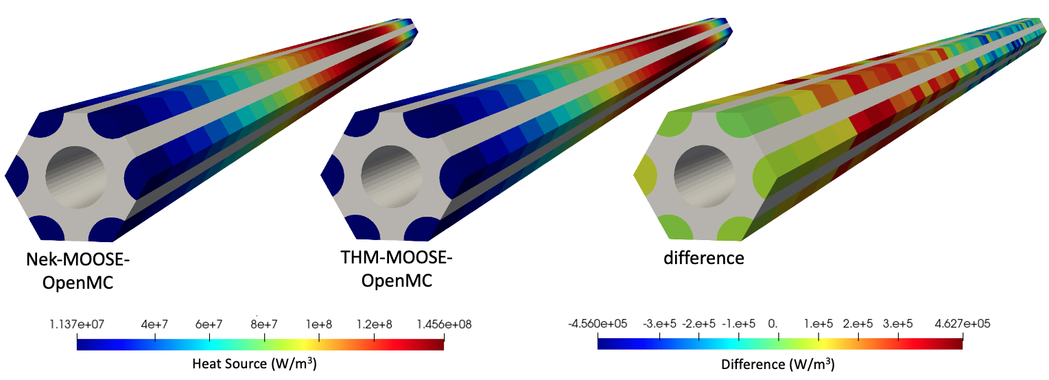
Figure 6: Heat source predicted by OpenMC with thermal feedback from either NekRS-MOOSE or THM-MOOSE
The lack of reflectors results in a relatively high leakage percentage of about 18.8%. For the unit cell, recall that the fluid temperature rise is only 82 K. These two effects combine to give a power distribution that is very nearly symmetric in the axial direction - while the lower solid temperatures near the inlet do cause power to shift slightly downwards, the magnitude of the shift is moderated by the effect of pushing the fission source closer to external boundaries, where those neutrons would be more likely to exit the domain.
In the earlier conjugate heat transfer tutorial, we showed that CHT calculations with NekRS-MOOSE and THM-MOOSE agree very well with one another in terms of fluid temperature, solid temperature, and fluid density. Especially when considering that the neutronics feedback due to fluid temperature and density are very small for gas-cooled systems, the excellent agreement in OpenMC's fission distribution shown in Figure 6 is as expected. When cast in terms of a percent difference (as opposed to the absolute difference shown in Figure 6), the NekRS-MOOSE-OpenMC and THM-MOOSE-OpenMC cases agree to within 1%, which is within the range of the uncertainty in the fission tally itself.
Figure 7 shows the solid temperature predicted by the MOOSE heat transfer module, with physics feedback provided by either NekRS-OpenMC or THM-OpenMC. The solid temperature peaks slightly downstream of the maximum OpenMC power due to the combined effects of the power distribution and convective heat transfer at the wall. Figure 7 helps explain the trend in the power difference shown in Figure 6. Near the inlet, NekRS predicts a lower temperature than THM, while near the outlet NekRS predicts a higher temperature than THM. Due to the negative temperature reactivity coefficient of the unit cell, this causes the NekRS-based coupled model to predict a higher power than THM near the inlet, but a lower power than THM near the outlet.
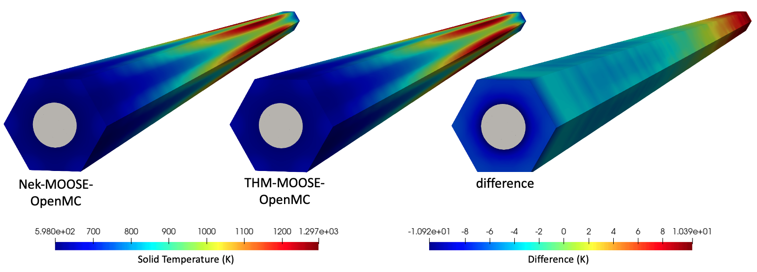
Figure 7: Solid temperature predicted by the MOOSE heat transfer module with physics feedback from either OpenMC-NekRS or OpenMC-THM.
Figure 8 shows the solid temperature predictions on the axial midplane with physics feedback provided by either NekRS-OpenMC or THM-OpenMC. Also shown is the difference between the two (NekRS-based case minus the THM-based case). The THM simulations are unable to capture the radial variation in heat flux along the channel wall, causing THM to underpredict temperatures near the channel wall close to the fuel compacts. However, an additional source of difference is now also present - small radial asymmetries in OpenMC's fission distribution contribute a small asymmetry in solid temperature on the order of 2 K. The tolerance on the fission power uncertainty can simply be increased in order to push down this contribution.
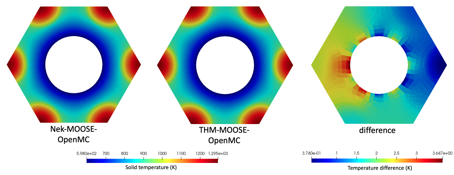
Figure 8: Solid temperature predicted by the MOOSE heat transfer module with physics feedback from either OpenMC-NekRS or OpenMC-THM on the axial mid-plane.
On each axial layer, the OpenMC model receives a total of 14 temperatures (six compacts plus six graphite regions around them, one graphite cell surrounding the coolant channel, and the coolant channel). Figure 9 shows the solid temperature predicted by the NekRS-MOOSE-OpenMC high-resolution simulations along with the actual cell temperature imposed in OpenMC for a half-height slice of the unit cell. OpenMC sets a volume-average temperature for each cell according to the mesh mirror element centroid mappings to OpenMC's cells.
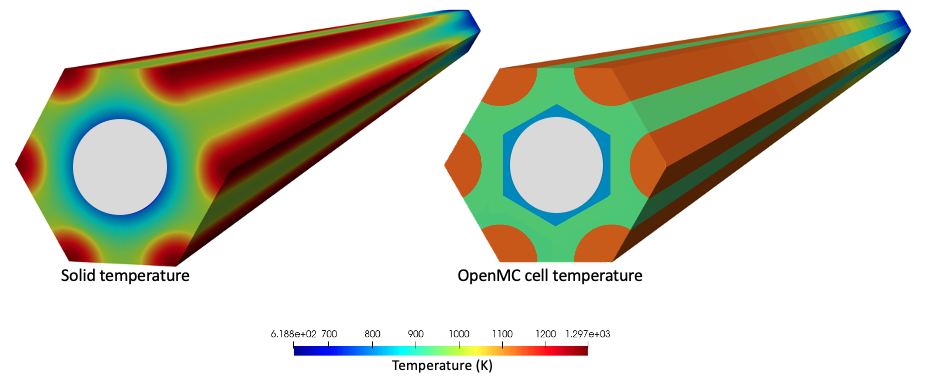
Figure 9: Solid temperature predicted by the MOOSE heat transfer module with physics feedback from OpenMC-NekRS and the solid temperature actually imposed in OpenMC for a half-height portion of the unit cell
Figure 10 shows the fluid temperature predicted by NekRS and THM, with physics feedback provided by MOOSE-OpenMC. NekRS resolves the thermal boundary layer, whereas the THM model uses the Dittus-Boelter correlation to represent the temperature drop from the heated wall to the bulk. Therefore, the fluid temperature shown in Figure 10 for THM is the area-averaged fluid temperature. The wall temperature predicted by NekRS follows a very similar distribution as the heat flux, with a profile that peaks slightly downstream of the maximum power due to the combined effects of convective heat transfer and the fission power distribution.
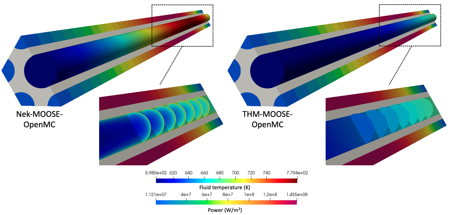
Figure 10: Fluid temperature predicted for the multiphysics simulations for NekRS-MOOSE-OpenMC and THM-MOOSE-OpenMC.
Figure 11 shows the radially-averaged temperatures for the two thermal-fluid feedback options. The fluid bulk temperature increases along the flow direction, with a faster rate of increase where the power density is highest.
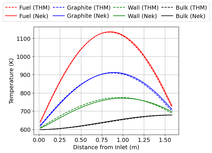
Figure 11: Radially-averaged temperatures for the NekRS-MOOSE-OpenMC and THM-MOOSE-OpenMC simulations.
References
- INL.
High-Temperature Gas-Cooled Test Reactor Point Design.
Technical Report INL/EXT-16-38296, Idaho National Laboratory, 2016.
URL: https://tinyurl.com/v9a4hym5.[Export]
- A.J. Novak, D. Andrs, P. Shriwise, J. Fang, H. Yuan, D. Shaver, E. Merzari, P.K. Romano, and R.C. Martineau.
Coupled Monte Carlo and Thermal-Fluid Modeling of High Temperature Gas Reactors Using Cardinal.
Annals of Nuclear Energy, 177:109310, 2022.
doi:10.1016/j.anucene.2022.109310.[Export]