Conjugate Heat Transfer for Turbulent Channel Flow
In this tutorial, you will learn how to:
Couple NekRS to MOOSE for CHT for turbulent flow in a Tri-Structural Isotropic (TRISO) fuel unit cell
Couple NekRS to MOOSE for solving NekRS in non-dimensional form
Extract an initial condition from a NekRS restart file
Swap out NekRS for a different thermal-fluid MOOSE application, the Thermal Hydraulics Module (THM)
Compute heat transfer coefficients with NekRS
To access this tutorial,
cd cardinal/tutorials/gas_compact_cht
This tutorial also requires you to download some mesh files from Box. Please download the files from the gas_compact_cht folder here and place these files within the same directory structure in tutorials/gas_compact_cht.
This tutorial was developed with support from the NEAMS Thermal Fluids Center of Excellence and the NRIC Virtual Test Bed (VTB). You can find additional context on this model in our journal article Novak et al. (2022).
This tutorial requires HPC resources to run the NekRS cases. Please still read this tutorial if you do not have resources, because you will be able to run the THM cases and much of the Cardinal usage is agnostic of the particular thermal code being used.
Geometry and Computational Model
The geometry consists of a unit cell of a TRISO-fueled gas reactor compact INL (2016). A top-down view of the geometry is shown in Figure 1. The fuel is cooled by helium flowing in a cylindrical channel of diameter . Cylindrical fuel compacts containing randomly-dispersed TRISO particles at 15% packing fraction are arranged around the coolant channel in a triangular lattice. The TRISO particles use a conventional design that consists of a central fissile uranium oxycarbide kernel enclosed in a carbon buffer, an inner Pyrolitic Carbon (PyC) layer, a silicon carbide layer, and finally an outer PyC layer. The geometric specifications are summarized in Table 1. Heat is produced in the TRISO particles to yield a total power of 38 kW.
-fueled gas reactor compact unit cell](../media/compact_unit_cell.png)
Figure 1: TRISO-fueled gas reactor compact unit cell
Table 1: Geometric specifications for a TRISO-fueled gas reactor compact
| Parameter | Value (cm) |
|---|---|
| Coolant channel diameter, | 1.6 |
| Fuel compact diameter, | 1.27 |
| Fuel-to-coolant center distance, | 1.628 |
| Height | 160 |
| TRISO kernel radius | 214.85e-4 |
| Buffer layer radius | 314.85e-4 |
| Inner PyC layer radius | 354.85e-4 |
| Silicon carbide layer radius | 389.85e-4 |
| Outer PyC layer radius | 429.85e-4 |
Heat Conduction Model
The MOOSE heat transfer module is used to solve for energy conservation in the solid, with the time derivative neglected in order to more quickly approach steady state. The solid mesh is shown in Figure 2. The TRISO particles are homogenized into the compact regions - all material properties in the heterogeneous regions are taken as volume averages of the various constituent materials.
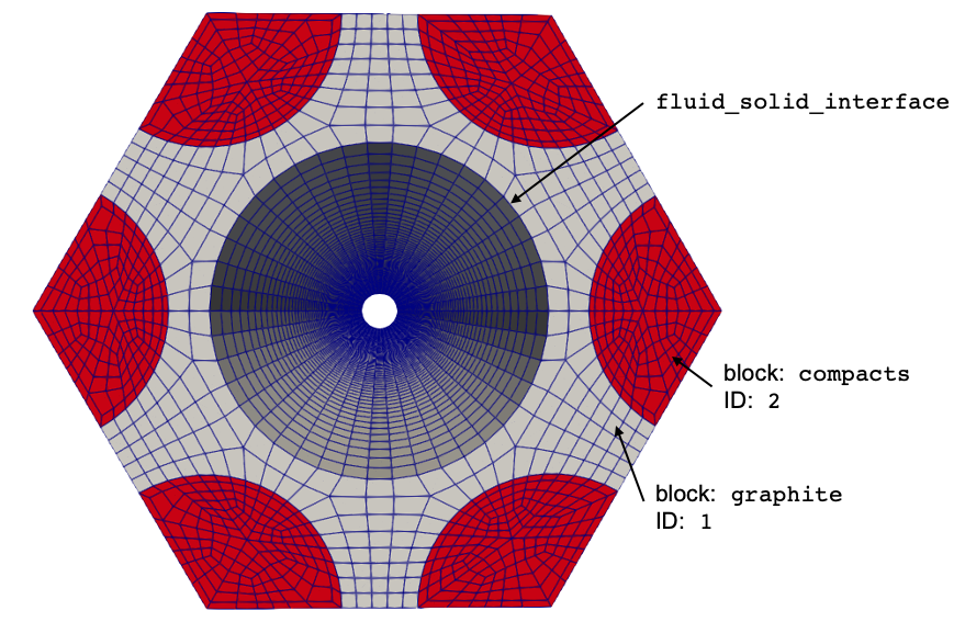
Figure 2: Mesh for the solid heat conduction model
The volumetric power density is set to a sinusoidal function of ,
where is a coefficient used to ensure that the total power produced is 38 kW and is the domain height. The power is uniform in the radial direction in each compact. On the coolant channel surface, a Dirichlet temperature is provided by NekRS/THM. All other boundaries are insulated. We will run the solid model first, so we must specify an initial condition for the wall temperature, which we simply set to a linear variation between the inlet and the outlet based on the nominal temperature rise.
NekRS Model
NekRS solves the incompressible k-tau RANS equations. To relate to , is selected. The resolution of the mesh near all no-slip boundaries ensures that such that the NekRS model is a wall-resolved model.
Here, the NekRS case will be set up in non-dimensional form. This is a convenient technique for fluid solvers, because the solution will be correct for any flow at a given Reynolds/Peclet/etc. number in this geometry. A common user operation is also to "ramp" up a CFD solve for stability purposes. Solving in non-dimensional form means that you do not need to also "ramp" absolute values for velocity/pressure/temperature/etc. - switching to a different set of non-dimensional numbers is as simple as just modifying the thermophysical "properties" of the fluid (e.g. viscosity, conductivity, etc.).
When the Navier-Stokes equations are written in non-dimensional form, the "density" in the [VELOCITY] block becomes unity because
(1)
The "viscosity" becomes the coefficient on the viscous stress term (, where is the Reynolds number). In NekRS, specifying diffusivity = -50.0 is equivalent to specifying diffusivity = 0.02 (i.e. ), or a Reynolds number of 50.0.
In non-dimensional form, the rhoCp term in the [TEMPERATURE] block becomes unity because
(2)
The "conductivity" indicates the coefficient on the diffusion kernel, which in non-dimensional form is equal to , where is the Peclet number. In NekRS, specifying conductivity = -35 is equivalent to specifying conductivity = 0.02857 (i.e. ), or a Peclet number of 35.
The inlet mass flowrate is 0.0905 kg/s; with the channel diameter of 1.6 cm and material properties of helium, this results in a Reynolds number of 223214 and a Prandtl number of 0.655. This highly-turbulent flow results in extremely thin momentum and thermal boundary layers on the no-slip surfaces forming the periphery of the coolant channel. In order to resolve the near-wall behavior, an extremely fine mesh is required in the NekRS simulation. To accelerate the overall coupled CHT case that is of interest in this tutorial, the NekRS model is split into a series of calculations:
We first run a partial-height, periodic flow-only case to obtain converged , , and distributions.
Then, we extrapolate the and to the full-height case.
Finally, we use the converged, full-height and distributions to transport a temperature passive scalar in a CHT calculation with MOOSE.
As a rough estimate, solving the coupled mass-momentum equations requires about an order of magnitude more compute time than a passive scalar equation in NekRS. Therefore, by "freezing" the and solutions, we can dramatically reduce the total cost of the coupled CHT calculation.
The periodic flow model has a height of and takes about 10,000 core hours to reach steady state. The extrapolation from to then is a simple postprocessing operation. Because steps 1 and 2 are done exclusively using NekRS, and the periodic flow solve takes a very long time to run (from the perspective of a tutorial, at least), we omit steps 1 and 2 from this tutorial. Instead, we begin straight away from a full-height periodic restart file with the - RANS model. This restart file is the periodic_flow_solve.f00001 file. If you open the restart file, you will see the following converged NekRS predictions of velocity, , and . Figure 4 shows the axial velocity, , and on a line plot through the center of the channel.

Figure 3: Converged NekRS predictions of velocity magnitude (left), (middle), and (right) for the periodic case (all in non-dimensional form)
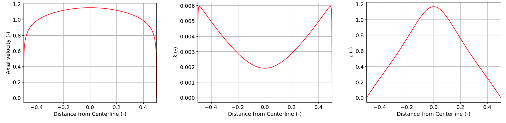
Figure 4: Converged NekRS predictions of velocity magnitude (left), (middle), and (right) for the periodic case along the channel mide-plane (all in non-dimensional form)
For the conjugate heat transfer case, we will load this restart file, compute from the loaded solutions for and , and then transport temperature with coupling to MOOSE heat conduction. The NekRS files are:
ranstube.re2: NekRS meshranstube.par: High-level settings for the solver, boundary condition mappings to sidesets, and the equations to solveranstube.udf: User-defined C++ functions for on-line postprocessing and model setupranstube.oudf: User-defined OCCA kernels for boundary conditions and source terms
The NekRS mesh is shown in Figure 5. Boundary 1 is the inlet, boundary 2 is the outlet, and boundary 3 is the wall. The same mesh was used for the periodic flow solve, except with a shorter height.
 model](../media/nek_mesh_uc.png)
Figure 5: Mesh for the NekRS RANS model
Next, the .par file contains problem setup information. This input sets up a nondimensional passive scalar solution, loading , , , and from a restart file. In order to "freeze," or turn off the , , , and solves, we set solver = none in the [VELOCITY], [SCALAR01] ( passive scalar), and [SCALAR02] ( passive scalar) blocks. The only equation that NekRS will solve is for temperature.
# Model of a turbulent channel flow.
#
# L_ref = 0.016 m          coolant channel diameter
# T_ref = 598 K            coolant inlet temperature
# dT_ref = 82.89 K         coolant nominal temperature rise in the unit cell
# U_ref = 81.089           coolant inlet velocity
# length = 1.6 m           coolant channel flow length
#
# rho_0 = 5.5508 kg/m3     coolant density
# mu_0 = 3.22639e-5 Pa-s   coolant dynamic viscosity
# Cp_0 = 5189 J/kg/K       coolant isobaric heat capacity
# k_0 = 0.2556 W/m/K       coolant thermal conductivity
#
# Re = 223214
# Pr = 0.655
# Pe = 146205

[GENERAL]
  startFrom = periodic_flow_solve.f00001

  polynomialOrder = 7
  dt = 6e-3
  timeStepper = BDF2

  stopAt = numSteps
  numSteps = 1000

  # write an output file every specified time steps
  writeControl = steps
  writeInterval = 1000

[PROBLEMTYPE]
  stressFormulation = true

[PRESSURE]
  residualTol = 1e-04

[VELOCITY]
  solver = none
  viscosity = -223214
  density = 1.0
  boundaryTypeMap = v, o, W
  residualTol = 1e-06

[TEMPERATURE]
  rhoCp = 1.0
  conductivity = -146205
  boundaryTypeMap = t, o, f
  residualTol = 1e-06

[SCALAR01] # k
  solver = none
  boundaryTypeMap = t, I, o
  residualTol = 1e-06
  rho = 1.0
  diffusivity = -223214

[SCALAR02] # tau
  solver = none
  boundaryTypeMap = t, I, o
  residualTol = 1e-06
  rho = 1.0
  diffusivity = -223214
Next, the .udf file is used to setup initial conditions and define how should be computed based on and the restart values of and . In turbulent_props, a user-defined function, we use from the input file in combination with the and (read from the restart file later in the .udf file) to adjust the total diffusion coefficient on temperature to according to the definition of turbulent Prandtl number. This adjustment must happen on device, in a new GPU kernel we name scalarScaledAddKernel. This kernel will be defined in the .oudf file; we instruct the JIT compilation to compile this new kernel by calling udfBuildKernel.
Then, in UDF_Setup we set an initial condition for fluid temperature (the first scalar in the nrs->cds->S array that holds all the scalars). In this function, we also store the value of computed in the restart file.
#include <math.h>
#include "udf.hpp"

occa::memory o_mu_t_from_restart;

#define length 100.0    // non-dimensional channel length
#define Pr_T 0.91       // turbulent Prandtl number

static occa::kernel scalarScaledAddKernel;

void turbulent_props(nrs_t *nrs, double time, occa::memory o_U, occa::memory o_S,
            occa::memory o_UProp, occa::memory o_SProp)
{
  // fetch the laminar thermal conductivity and specify the desired turbulent Pr
  dfloat k_laminar;
  platform->options.getArgs("SCALAR00 DIFFUSIVITY", k_laminar);

  // o_diff is the turbulent conductivity for all passive scalars, so we grab the first
  // slice, since temperature is the first passive scalar
  occa::memory o_mu = nrs->cds->o_diff + 0 * nrs->cds->fieldOffset[0] * sizeof(dfloat);

  scalarScaledAddKernel(0, nrs->cds->mesh[0]->Nlocal, k_laminar, 1.0 / Pr_T,
    o_mu_t_from_restart /* turbulent viscosity */, o_mu /* laminar viscosity */);
}

void UDF_LoadKernels(occa::properties & kernelInfo)
{
  scalarScaledAddKernel = oudfBuildKernel(kernelInfo, "scalarScaledAdd");
}

void UDF_Setup(nrs_t *nrs)
{
  mesh_t *mesh = nrs->cds->mesh[0];
  int n_gll_points = mesh->Np * mesh->Nelements;

  // allocate space for the k and tau that we will read from the file
  dfloat * mu_t = (dfloat *) calloc(n_gll_points, sizeof(dfloat));

  for (int n = 0; n < n_gll_points; ++n)
  {
    // initialize the temperature to a linear variation from 0 to 1
    dfloat z = mesh->z[n];
    nrs->cds->S[n + 0 * nrs->cds->fieldOffset[0]] = z / length;

    // fetch the restart value of mu_T, which is equal to k * tau, the second and third
    // passive scalars
    mu_t[n] = nrs->cds->S[n + 1 * nrs->cds->fieldOffset[0]] *
              nrs->cds->S[n + 2 * nrs->cds->fieldOffset[0]];
  }

  o_mu_t_from_restart = platform->device.malloc(n_gll_points * sizeof(dfloat), mu_t);

  udf.properties = &turbulent_props;
}

void UDF_ExecuteStep(nrs_t * nrs, double time, int tstep)
{
}
In the .oudf file, we define boundary conditions for temperature and also the form of the scalarScaledAdd kernel that we use to compute . The inlet boundary is set to a temperature of 0 (a dimensional temperature of ), while the fluid-solid interface will receive a heat flux from MOOSE.
@kernel void scalarScaledAdd(const dlong offset, const dlong N,
                             const dfloat a,
                             const dfloat b,
                             @restrict const dfloat* X,
                             @restrict dfloat* Y)
{
  for (dlong n = 0; n < N; ++n; @tile(256,@outer,@inner))
    if (n < N)
      Y[n] = a + b * X[n + offset];
}

// Boundary conditions are only needed for temperature, since the solves of pressure,
// velocity, k, and tau are all frozen

void scalarDirichletConditions(bcData *bc)
{
  // inlet temperature
  bc->s = 0.0;
}

void scalarNeumannConditions(bcData *bc)
{
  // wall (temperature)
  // note: when running with Cardinal, Cardinal will allocate the usrwrk
  // array. If running with NekRS standalone (e.g. nrsmpi), you need to
  // replace the usrwrk with some other value or allocate it youself from
  // the udf and populate it with values.
  bc->flux = bc->usrwrk[bc->idM];
}
THM Model
THM solves the 1-D area averages of the Navier-Stokes equations. The Churchill correlation is used for and the Dittus-Boelter correlation is used for Berry et al. (2014).
The THM mesh contains 150 elements; the mesh is constucted automatically within THM. The heat flux imposed in the THM elements is obtained by area averaging the heat flux from the heat conduction model in 150 layers along the fluid-solid interface. For the reverse transfer, the wall temperature sent to MOOSE heat conduction is set to a uniform value along the fluid-solid interface according to a nearest-node mapping to the THM elements.
Because the thermal-fluids tools run after the MOOSE heat conduction application, initial conditions are only required for pressure, fluid temperature, and velocity, which are set to uniform distributions.
CHT Coupling
In this section, MOOSE, NekRS, and THM are coupled for CHT. Two separate simulations are performed here:
Coupling of NekRS with MOOSE
Coupling of THM with MOOSE
By individually describing the two setups, you will understand that NekRS is really as interchangeable as any other MOOSE application for coupling. In addition, we will describe how to generate a heat transfer coefficient from the NekRS-MOOSE coupling to input into the THM-MOOSE coupling to demonstrate an important multiscale use case of NekRS.
NekRS-MOOSE
In this section, we describe the coupling of MOOSE and NekRS.
Solid Input Files
The solid phase is solved with the MOOSE heat transfer module, and is described in the solid_nek.i input. We define a number of constants at the beginning of the file and set up the mesh.
!include common_input.i

# This input models conjugate heat transfer between MOOSE and NekRS for
# a single coolant channel. This input file should be run with:
#
# cardinal-opt -i solid_nek.i

unit_cell_power = ${fparse power / (n_bundles * n_coolant_channels_per_block) * unit_cell_height / height}
unit_cell_mdot = ${fparse mdot / (n_bundles * n_coolant_channels_per_block)}

# compute the volume fraction of each TRISO layer in a TRISO particle
# for use in computing average thermophysical properties
kernel_fraction = ${fparse kernel_radius^3 / oPyC_radius^3}
buffer_fraction = ${fparse (buffer_radius^3 - kernel_radius^3) / oPyC_radius^3}
ipyc_fraction = ${fparse (iPyC_radius^3 - buffer_radius^3) / oPyC_radius^3}
sic_fraction = ${fparse (SiC_radius^3 - iPyC_radius^3) / oPyC_radius^3}
opyc_fraction = ${fparse (oPyC_radius^3 - SiC_radius^3) / oPyC_radius^3}

# multiplicative factor on assumed heat source distribution to get correct magnitude
q0 = ${fparse unit_cell_power / (4.0 * unit_cell_height * compact_diameter * compact_diameter / 4.0)}

# Time step interval on which to exchange data between NekRS and MOOSE
N = 50
U_ref = ${fparse mdot / (n_bundles * n_coolant_channels_per_block) / fluid_density / (pi * channel_diameter * channel_diameter / 4.0)}
t0 = ${fparse channel_diameter / U_ref}
nek_dt = 6e-3

[Mesh]
  type = FileMesh
  file = solid_rotated.e
[]
Next, we define a temperature variable T, and specify the governing equations and boundary conditions we will apply.
[Variables<<<{"href": "../syntax/Variables/index.html"}>>>]
  [T]
    initial_condition<<<{"description": "Specifies a constant initial condition for this variable"}>>> = ${inlet_T}
  []
[]

[Kernels<<<{"href": "../syntax/Kernels/index.html"}>>>]
  [diffusion]
    type = HeatConduction<<<{"description": "Diffusive heat conduction term $-\\nabla\\cdot(k\\nabla T)$ of the thermal energy conservation equation", "href": "../source/kernels/HeatConduction.html"}>>>
    variable<<<{"description": "The name of the variable that this residual object operates on"}>>> = T
  []
  [source]
    type = CoupledForce<<<{"description": "Implements a source term proportional to the value of a coupled variable. Weak form: $(\\psi_i, -\\sigma v)$.", "href": "../source/kernels/CoupledForce.html"}>>>
    variable<<<{"description": "The name of the variable that this residual object operates on"}>>> = T
    v<<<{"description": "The coupled variable which provides the force"}>>> = power
    block<<<{"description": "The list of blocks (ids or names) that this object will be applied"}>>> = 'compacts'
  []
[]

[BCs<<<{"href": "../syntax/BCs/index.html"}>>>]
  [pin_outer]
    type = MatchedValueBC<<<{"description": "Implements a NodalBC which equates two different Variables' values on a specified boundary.", "href": "../source/bcs/MatchedValueBC.html"}>>>
    variable<<<{"description": "The name of the variable that this residual object operates on"}>>> = T
    v<<<{"description": "The variable whose value we are to match."}>>> = fluid_temp
    boundary<<<{"description": "The list of boundary IDs from the mesh where this object applies"}>>> = 'fluid_solid_interface'
  []
[]

[ICs<<<{"href": "../syntax/Cardinal/ICs/index.html"}>>>]
  [power]
    type = FunctionIC<<<{"description": "An initial condition that uses a normal function of x, y, z to produce values (and optionally gradients) for a field variable.", "href": "../source/ics/FunctionIC.html"}>>>
    variable<<<{"description": "The variable this initial condition is supposed to provide values for."}>>> = power
    function<<<{"description": "The initial condition function."}>>> = axial_power
    block<<<{"description": "The list of blocks (ids or names) that this object will be applied"}>>> = 'compacts'
  []
  [fluid_temp]
    type = FunctionIC<<<{"description": "An initial condition that uses a normal function of x, y, z to produce values (and optionally gradients) for a field variable.", "href": "../source/ics/FunctionIC.html"}>>>
    variable<<<{"description": "The variable this initial condition is supposed to provide values for."}>>> = fluid_temp
    function<<<{"description": "The initial condition function."}>>> = axial_fluid_temp
  []
[]The MOOSE heat transfer module will receive a wall temperature from NekRS in the form of an AuxVariable, so we define a receiver variable for the temperature, as fluid_temp. The MOOSE heat transfer module will also send heat flux to NekRS, which we compute as another AuxVariable named flux, which we compute with a DiffusionFluxAux auxiliary kernel. Finally, we define another auxiliary variable for the imposed power.
[AuxVariables<<<{"href": "../syntax/AuxVariables/index.html"}>>>]
  [fluid_temp]
  []
  [flux]
    family<<<{"description": "Specifies the family of FE shape functions to use for this variable"}>>> = MONOMIAL
    order<<<{"description": "Specifies the order of the FE shape function to use for this variable (additional orders not listed are allowed)"}>>> = CONSTANT
  []
  [power]
    family<<<{"description": "Specifies the family of FE shape functions to use for this variable"}>>> = MONOMIAL
    order<<<{"description": "Specifies the order of the FE shape function to use for this variable (additional orders not listed are allowed)"}>>> = CONSTANT
  []
[]

[AuxKernels<<<{"href": "../syntax/AuxKernels/index.html"}>>>]
  [flux]
    type = DiffusionFluxAux<<<{"description": "Compute components of flux vector for diffusion problems $(\\vec{J} = -D \\nabla C)$.", "href": "../source/auxkernels/DiffusionFluxAux.html"}>>>
    diffusion_variable<<<{"description": "The name of the variable"}>>> = T
    component<<<{"description": "The desired component of flux."}>>> = normal
    diffusivity<<<{"description": "The name of the diffusivity material property that will be used in the flux computation."}>>> = thermal_conductivity
    variable<<<{"description": "The name of the variable that this object applies to"}>>> = flux
    boundary<<<{"description": "The list of boundaries (ids or names) from the mesh where this object applies"}>>> = 'fluid_solid_interface'
  []
[]Next, we use functions to define the thermal conductivities. The material properties for the TRISO compacts are taken as volume averages of the various constituent materials. We also use functions to set initial conditions for power (a sinusoidal function) and the initial fluid temperature (a linear variation from inlet to outlet).
[Functions<<<{"href": "../syntax/Functions/index.html"}>>>]
  [k_graphite]
    type = ParsedFunction<<<{"description": "Function created by parsing a string", "href": "../source/functions/MooseParsedFunction.html"}>>>
    expression<<<{"description": "The user defined function."}>>> = '${matrix_k}'
  []
  [k_TRISO]
    type = ParsedFunction<<<{"description": "Function created by parsing a string", "href": "../source/functions/MooseParsedFunction.html"}>>>
    expression<<<{"description": "The user defined function."}>>> = '${kernel_fraction} * ${kernel_k} + ${buffer_fraction} * ${buffer_k} + ${fparse ipyc_fraction + opyc_fraction} * ${PyC_k} + ${sic_fraction} * ${SiC_k}'
  []
  [k_compacts]
    type = ParsedFunction<<<{"description": "Function created by parsing a string", "href": "../source/functions/MooseParsedFunction.html"}>>>
    expression<<<{"description": "The user defined function."}>>> = '${triso_pf} * k_TRISO + ${fparse 1.0 - triso_pf} * k_graphite'
    symbol_names<<<{"description": "Symbols (excluding t,x,y,z) that are bound to the values provided by the corresponding items in the symbol_values vector."}>>> = 'k_TRISO k_graphite'
    symbol_values<<<{"description": "Constant numeric values, postprocessor names, function names, and scalar variables corresponding to the symbols in symbol_names."}>>> = 'k_TRISO k_graphite'
  []
  [axial_power] # volumetric power density
    type = ParsedFunction<<<{"description": "Function created by parsing a string", "href": "../source/functions/MooseParsedFunction.html"}>>>
    expression<<<{"description": "The user defined function."}>>> = 'sin(pi * z / ${unit_cell_height}) * ${q0}'
  []
  [axial_fluid_temp]
    type = ParsedFunction<<<{"description": "Function created by parsing a string", "href": "../source/functions/MooseParsedFunction.html"}>>>
    expression<<<{"description": "The user defined function."}>>> = '${inlet_T} + z / ${unit_cell_height} * ${unit_cell_power} / ${unit_cell_mdot} / ${fluid_Cp}'
  []
[]

[Materials<<<{"href": "../syntax/Materials/index.html"}>>>]
  [graphite]
    type = HeatConductionMaterial<<<{"description": "General-purpose material model for heat conduction", "href": "../source/materials/HeatConductionMaterial.html"}>>>
    thermal_conductivity_temperature_function<<<{"description": "Thermal conductivity as a function of temperature."}>>> = k_graphite
    temp = T
    block<<<{"description": "The list of blocks (ids or names) that this object will be applied"}>>> = 'graphite'
  []
  [compacts]
    type = HeatConductionMaterial<<<{"description": "General-purpose material model for heat conduction", "href": "../source/materials/HeatConductionMaterial.html"}>>>
    thermal_conductivity_temperature_function<<<{"description": "Thermal conductivity as a function of temperature."}>>> = k_compacts
    temp = T
    block<<<{"description": "The list of blocks (ids or names) that this object will be applied"}>>> = 'compacts'
  []
[]We define a number of postprocessors for querying the solution as well as for normalizing the heat flux.
[Postprocessors<<<{"href": "../syntax/Postprocessors/index.html"}>>>]
  [flux_integral]
    # evaluate the total heat flux for normalization
    type = SideDiffusiveFluxIntegral<<<{"description": "Computes the integral of the diffusive flux over the specified boundary", "href": "../source/postprocessors/SideDiffusiveFluxIntegral.html"}>>>
    diffusivity<<<{"description": "The name of the diffusivity material property that will be used in the flux computation. This must be provided if the variable is of finite element type"}>>> = thermal_conductivity
    variable<<<{"description": "The name of the variable which this postprocessor integrates"}>>> = T
    boundary<<<{"description": "The list of boundary IDs from the mesh where this object applies"}>>> = 'fluid_solid_interface'
  []
  [max_fuel_T]
    type = ElementExtremeValue<<<{"description": "Finds either the min or max elemental value of a variable over the domain.", "href": "../source/postprocessors/ElementExtremeValue.html"}>>>
    variable<<<{"description": "The name of the variable that this postprocessor operates on"}>>> = T
    value_type<<<{"description": "Type of extreme value to return. 'max' returns the maximum value. 'min' returns the minimum value. 'max_abs' returns the maximum of the absolute value."}>>> = max
    block<<<{"description": "The list of blocks (ids or names) that this object will be applied"}>>> = 'compacts'
  []
  [max_block_T]
    type = ElementExtremeValue<<<{"description": "Finds either the min or max elemental value of a variable over the domain.", "href": "../source/postprocessors/ElementExtremeValue.html"}>>>
    variable<<<{"description": "The name of the variable that this postprocessor operates on"}>>> = T
    value_type<<<{"description": "Type of extreme value to return. 'max' returns the maximum value. 'min' returns the minimum value. 'max_abs' returns the maximum of the absolute value."}>>> = max
    block<<<{"description": "The list of blocks (ids or names) that this object will be applied"}>>> = 'graphite'
  []
  [max_flux]
    type = ElementExtremeValue<<<{"description": "Finds either the min or max elemental value of a variable over the domain.", "href": "../source/postprocessors/ElementExtremeValue.html"}>>>
    variable<<<{"description": "The name of the variable that this postprocessor operates on"}>>> = flux
  []
  [synchronization_to_nek]
    type = Receiver<<<{"description": "Reports the value stored in this processor, which is usually filled in by another object. The Receiver does not compute its own value.", "href": "../source/postprocessors/Receiver.html"}>>>
    default<<<{"description": "The default value"}>>> = 1.0
  []

  [power]
    type = ElementIntegralVariablePostprocessor<<<{"description": "Computes a volume integral of the specified variable", "href": "../source/postprocessors/ElementIntegralVariablePostprocessor.html"}>>>
    variable<<<{"description": "The name of the variable that this object operates on"}>>> = power
    block<<<{"description": "The list of blocks (ids or names) that this object will be applied"}>>> = 'compacts'
  []
[]For visualization purposes only, we add LayeredAverages to average the fuel and block temperatures in layers in the direction. We also add a LayeredSideAverage to average the heat flux along a boundary, again in layers in the direction. We then output the results of these userobjects to CSV using SpatialUserObjectVectorPostprocessors and by setting csv = true in the output.
[UserObjects<<<{"href": "../syntax/UserObjects/index.html"}>>>]
  [average_fuel_axial]
    type = LayeredAverage<<<{"description": "Computes averages of variables over layers", "href": "../source/userobjects/LayeredAverage.html"}>>>
    variable<<<{"description": "The name of the variable that this object operates on"}>>> = T
    direction<<<{"description": "The direction of the layers."}>>> = z
    num_layers<<<{"description": "The number of layers."}>>> = ${num_layers_for_plots}
    block<<<{"description": "The list of block ids (SubdomainID) that this object will be applied"}>>> = 'compacts'
  []
  [average_block_axial]
    type = LayeredAverage<<<{"description": "Computes averages of variables over layers", "href": "../source/userobjects/LayeredAverage.html"}>>>
    variable<<<{"description": "The name of the variable that this object operates on"}>>> = T
    direction<<<{"description": "The direction of the layers."}>>> = z
    num_layers<<<{"description": "The number of layers."}>>> = ${num_layers_for_plots}
    block<<<{"description": "The list of block ids (SubdomainID) that this object will be applied"}>>> = 'graphite'
  []
  [average_flux_axial]
    type = LayeredSideAverage<<<{"description": "Computes side averages of a variable storing partial sums for the specified number of intervals in a direction (x,y,z).", "href": "../source/userobjects/LayeredSideAverage.html"}>>>
    variable<<<{"description": "The name of the variable that this boundary condition applies to"}>>> = flux
    direction<<<{"description": "The direction of the layers."}>>> = z
    num_layers<<<{"description": "The number of layers."}>>> = ${num_layers_for_plots}
    boundary<<<{"description": "The list of boundary IDs from the mesh where this object applies"}>>> = 'fluid_solid_interface'
  []
[]

[VectorPostprocessors<<<{"href": "../syntax/VectorPostprocessors/index.html"}>>>]
  [fuel_axial_avg]
    type = SpatialUserObjectVectorPostprocessor<<<{"description": "Outputs the values of a spatial user object in the order of the specified spatial points", "href": "../source/vectorpostprocessors/SpatialUserObjectVectorPostprocessor.html"}>>>
    userobject<<<{"description": "The userobject whose values are to be reported"}>>> = average_fuel_axial
  []
  [block_axial_avg]
    type = SpatialUserObjectVectorPostprocessor<<<{"description": "Outputs the values of a spatial user object in the order of the specified spatial points", "href": "../source/vectorpostprocessors/SpatialUserObjectVectorPostprocessor.html"}>>>
    userobject<<<{"description": "The userobject whose values are to be reported"}>>> = average_block_axial
  []
  [flux_axial_avg]
    type = SpatialUserObjectVectorPostprocessor<<<{"description": "Outputs the values of a spatial user object in the order of the specified spatial points", "href": "../source/vectorpostprocessors/SpatialUserObjectVectorPostprocessor.html"}>>>
    userobject<<<{"description": "The userobject whose values are to be reported"}>>> = average_flux_axial
  []
[]

[Outputs<<<{"href": "../syntax/Outputs/index.html"}>>>]
  exodus<<<{"description": "Output the results using the default settings for Exodus output."}>>> = true
  print_linear_residuals<<<{"description": "Enable printing of linear residuals to the screen (Console)"}>>> = false
  hide<<<{"description": "A list of the variables and postprocessors that should NOT be output to the Exodus file (may include Variables, ScalarVariables, and Postprocessor names)."}>>> = 'synchronization_to_nek'

  [csv]
    file_base<<<{"description": "The desired solution output name without an extension. If not provided, MOOSE sets it with Outputs/file_base when available. Otherwise, MOOSE uses input file name and this object name for a master input or uses master file_base, the subapp name and this object name for a subapp input to set it."}>>> = 'csv/solid_nek'
    type = CSV<<<{"description": "Output for postprocessors, vector postprocessors, and scalar variables using comma seperated values (CSV).", "href": "../source/outputs/CSV.html"}>>>
  []
[]Finally, we add a TransientMultiApp that will run a MOOSE-wrapped NekRS simulation. Then, we add four different transfers to/from NekRS:
MultiAppGeneralFieldNearestLocationTransfer to send the heat flux from MOOSE to NekRS
MultiAppGeneralFieldNearestLocationTransfer to send temperature from NekRS to MOOSE
MultiAppPostprocessorTransfer to normalize the heat flux sent to NekRS (this is used internally by NekBoundaryFlux in the NekRS-wrapped input file)
MultiAppPostprocessorTransfer to send a dummy postprocessor named
synchronization_to_nekthat simply allows the NekRS sub-application to know when "new" coupling data is available from MOOSE, and to only do transfers to/from GPU when new data is available; please consult the NekRSProblem documentation for further information.
[MultiApps<<<{"href": "../syntax/MultiApps/index.html"}>>>]
  [nek]
    type = TransientMultiApp<<<{"description": "MultiApp for performing coupled simulations with the parent and sub-application both progressing in time.", "href": "../source/multiapps/TransientMultiApp.html"}>>>
    input_files<<<{"description": "The input file for each App.  If this parameter only contains one input file it will be used for all of the Apps.  When using 'positions_from_file' it is also admissable to provide one input_file per file."}>>> = 'nek.i'
    sub_cycling<<<{"description": "Set to true to allow this MultiApp to take smaller timesteps than the rest of the simulation.  More than one timestep will be performed for each parent application timestep"}>>> = true
    execute_on<<<{"description": "The list of flag(s) indicating when this object should be executed. For a description of each flag, see https://mooseframework.inl.gov/source/interfaces/SetupInterface.html."}>>> = timestep_end
  []
[]

[Transfers<<<{"href": "../syntax/Transfers/index.html"}>>>]
  [heat_flux_to_nek]
    type = MultiAppGeneralFieldNearestLocationTransfer<<<{"description": "Transfers field data at the MultiApp position by finding the value at the nearest neighbor(s) in the origin application.", "href": "../source/transfers/MultiAppGeneralFieldNearestLocationTransfer.html"}>>>
    source_variable<<<{"description": "The variable to transfer from."}>>> = flux
    variable<<<{"description": "The auxiliary variable to store the transferred values in."}>>> = flux
    from_boundaries<<<{"description": "The boundary we are transferring from (if not specified, whole domain is used)."}>>> = 'fluid_solid_interface'
    to_boundaries<<<{"description": "The boundary we are transferring to (if not specified, whole domain is used)."}>>> = '3'
    to_multi_app<<<{"description": "The name of the MultiApp to transfer the data to"}>>> = nek
  []
  [flux_integral_to_nek]
    type = MultiAppPostprocessorTransfer<<<{"description": "Transfers postprocessor data between the master application and sub-application(s).", "href": "../source/transfers/MultiAppPostprocessorTransfer.html"}>>>
    to_postprocessor<<<{"description": "The name of the Postprocessor in the MultiApp to transfer the value to.  This should most likely be a Reporter Postprocessor."}>>> = flux_integral
    from_postprocessor<<<{"description": "The name of the Postprocessor in the Master to transfer the value from."}>>> = flux_integral
    to_multi_app<<<{"description": "The name of the MultiApp to transfer the data to"}>>> = nek
  []
  [temperature_to_bison]
    type = MultiAppGeneralFieldNearestLocationTransfer<<<{"description": "Transfers field data at the MultiApp position by finding the value at the nearest neighbor(s) in the origin application.", "href": "../source/transfers/MultiAppGeneralFieldNearestLocationTransfer.html"}>>>
    source_variable<<<{"description": "The variable to transfer from."}>>> = temperature
    variable<<<{"description": "The auxiliary variable to store the transferred values in."}>>> = fluid_temp
    from_boundaries<<<{"description": "The boundary we are transferring from (if not specified, whole domain is used)."}>>> = '3'
    to_boundaries<<<{"description": "The boundary we are transferring to (if not specified, whole domain is used)."}>>> = 'fluid_solid_interface'
    from_multi_app<<<{"description": "The name of the MultiApp to receive data from"}>>> = nek
  []
  [synchronization_to_nek]
    type = MultiAppPostprocessorTransfer<<<{"description": "Transfers postprocessor data between the master application and sub-application(s).", "href": "../source/transfers/MultiAppPostprocessorTransfer.html"}>>>
    to_postprocessor<<<{"description": "The name of the Postprocessor in the MultiApp to transfer the value to.  This should most likely be a Reporter Postprocessor."}>>> = transfer_in
    from_postprocessor<<<{"description": "The name of the Postprocessor in the Master to transfer the value from."}>>> = synchronization_to_nek
    to_multi_app<<<{"description": "The name of the MultiApp to transfer the data to"}>>> = nek
  []
[]Finally, although our heat conduction model does not have any time derivatives (in order to more quickly reach steady state), NekRS must be run as a transient. In order to control the interval on which NekRS couples to MOOSE, we use a MOOSE time step that is N times bigger than the NekRS time step, taking care to account for the fact that the time step in the ranstube.par file is actually a nondimensional time step. By setting subcycling = true for the TransientMultiApp, MOOSE is only run every N time steps (the subcycling setting), and that the NekRS solution is only copied to/from GPU every N time steps (the minimize transfers setting).
Finally, we will run the MOOSE heat conduction model until the relative change in the solution (across the entire domain) differs by less than from the previous time step. While this may seem like a large tolerance, because the difference is taken over the entire domain, you will see changes only on the order of the fourth or fifth decimal place in temperatures.
[Executioner<<<{"href": "../syntax/Executioner/index.html"}>>>]
  type = Transient
  dt = '${fparse N * nek_dt * t0}'

  nl_abs_tol = 1e-5
  nl_rel_tol = 1e-16
  petsc_options_value = 'hypre boomeramg'
  petsc_options_iname = '-pc_type -pc_hypre_type'

  steady_state_detection = true
  steady_state_tolerance = 1e-1
[]Fluid Input Files
The Nek wrapping is described in the nek.i input file. We first define a few file-local variables, and then build a mesh mirror with a NekRSMesh. By setting boundary = '3', we indicate that boundary 3 will be coupled via CHT. In this example, we don't have any volume-based coupling, but we set volume = true to visualize the NekRS solution in Exodus format (as a first-order interpolation of the 7-th order polynomial solution).
When solving in MOOSE, all the coupled applications must either be in non-dimensional form, or all in dimensional form. In this tutorial, we have set up the MOOSE input file in dimensional form, but the NekRS case files were set up in non-dimensional form. In order for MOOSE's transfers to correctly find the closest nodes in the solid mesh to corresponding locations in NekRS, the entire mesh "mirror" through which data transfers occur must be scaled by a factor of to return to dimensional units (because the coupled MOOSE application is in dimensional units). This scaling is specified by the scaling parameter. In other words, the scaling indicates by what factor we should internally scale spatial lengths by to correctly send data between NekRS and MOOSE.
!include common_input.i

[Mesh]
  type = NekRSMesh
  boundary = '3'
  volume = true
  scaling = ${channel_diameter}
[]
Next, we define additional parameters to describe how NekRS interacts with MOOSE with the NekRSProblem. To allow conversion between a non-dimensional NekRS solve and a dimensional MOOSE coupled heat conduction application, the characteristic scales used to establish the non-dimensional problem are provided. Definitions for these non-dimensional scales are available here.
These characteristic scales are used by Cardinal to dimensionalize the NekRS solution into the units that the coupled MOOSE application expects. You still need to properly non-dimensionalize the NekRS input files (to be discussed later).
We also indicate that we are going to restrict the data copies to/from GPU to only occur on the time steps that NekRS is coupled to MOOSE. Then, we add the field transfers to send heat flux into NekRS, by reading from an auxiliary variable named flux with NekBoundaryFlux. We fetch the temperature from NekRS using a NekFieldVariable.
[Problem<<<{"href": "../syntax/Problem/index.html"}>>>]
  type = NekRSProblem
  casename<<<{"description": "Case name for the NekRS input files; this is <case> in <case>.par, <case>.udf, <case>.oudf, and <case>.re2."}>>> = 'ranstube'
  n_usrwrk_slots<<<{"description": "Number of slots to allocate in nrs->usrwrk to hold fields either related to coupling (which will be populated by Cardinal), or other custom usages, such as a distance-to-wall calculation"}>>> = 1

  [Dimensionalize<<<{"href": "../syntax/Problem/Dimensionalize/index.html"}>>>]
    U<<<{"description": "Reference velocity"}>>> = '${fparse mdot / (n_bundles * n_coolant_channels_per_block) / fluid_density / (pi * channel_diameter * channel_diameter / 4.0)}'
    T<<<{"description": "Reference temperature"}>>> = ${inlet_T}
    dT<<<{"description": "Reference temperature difference"}>>> = '${fparse power / mdot / fluid_Cp * unit_cell_height / height}'
    L<<<{"description": "Reference length"}>>> = ${channel_diameter}
    rho<<<{"description": "Reference density"}>>> = ${fluid_density}
    Cp<<<{"description": "Reference isobaric specific heat"}>>> = ${fluid_Cp}
  []

  [FieldTransfers<<<{"href": "../syntax/Problem/FieldTransfers/index.html"}>>>]
    [flux]
      type = NekBoundaryFlux<<<{"description": "Reads/writes boundary flux data between NekRS and MOOSE."}>>>
      direction<<<{"description": "Direction in which to send data"}>>> = to_nek
      usrwrk_slot<<<{"description": "When 'direction = to_nek', the slot(s) in the usrwrk array to write the incoming data; provide one entry for each quantity being passed"}>>> = 0
    []
    [temperature]
      type = NekFieldVariable<<<{"description": "Reads/writes volumetric field data between NekRS and MOOSE."}>>>
      direction<<<{"description": "Direction in which to send data"}>>> = from_nek
    []
  []

  synchronization_interval = parent_app
[]For time stepping, we will allow NekRS to control its own time stepping by using the NekTimeStepper. We will output both Exodus and CSV format data as well.
[Executioner<<<{"href": "../syntax/Executioner/index.html"}>>>]
  type = Transient

  [TimeStepper<<<{"href": "../syntax/Executioner/TimeStepper/index.html"}>>>]
    type = NekTimeStepper
    min_dt = 1e-10
  []
[]

[Outputs<<<{"href": "../syntax/Outputs/index.html"}>>>]
  exodus<<<{"description": "Output the results using the default settings for Exodus output."}>>> = true

  [screen]
    type = Console<<<{"description": "Object for screen output.", "href": "../source/outputs/Console.html"}>>>
    hide<<<{"description": "A list of the variables and postprocessors that should NOT be output to the Exodus file (may include Variables, ScalarVariables, and Postprocessor names)."}>>> = 'boundary_flux inlet_T outlet_T max_T flux_integral transfer_in'
  []

  [csv]
    file_base<<<{"description": "The desired solution output name without an extension. If not provided, MOOSE sets it with Outputs/file_base when available. Otherwise, MOOSE uses input file name and this object name for a master input or uses master file_base, the subapp name and this object name for a subapp input to set it."}>>> = 'csv/nek'
    type = CSV<<<{"description": "Output for postprocessors, vector postprocessors, and scalar variables using comma seperated values (CSV).", "href": "../source/outputs/CSV.html"}>>>
  []
[]Then, we define a few postprocessors to use for querying the solution. While we hide these from the console output above, they will still be output to CSV.
[Postprocessors<<<{"href": "../syntax/Postprocessors/index.html"}>>>]
  [boundary_flux]
    type = NekHeatFluxIntegral<<<{"description": "Heat flux over a boundary in the NekRS mesh", "href": "../source/postprocessors/NekHeatFluxIntegral.html"}>>>
    boundary<<<{"description": "Boundary ID(s) for which to compute the postprocessor"}>>> = '3'
  []
  [inlet_T]
    type = NekSideAverage<<<{"description": "Average of a field over a boundary of the NekRS mesh", "href": "../source/postprocessors/NekSideAverage.html"}>>>
    field<<<{"description": "Field to apply this object to"}>>> = temperature
    boundary<<<{"description": "Boundary ID(s) for which to compute the postprocessor"}>>> = '1'
  []
  [outlet_T]
    type = NekSideAverage<<<{"description": "Average of a field over a boundary of the NekRS mesh", "href": "../source/postprocessors/NekSideAverage.html"}>>>
    field<<<{"description": "Field to apply this object to"}>>> = temperature
    boundary<<<{"description": "Boundary ID(s) for which to compute the postprocessor"}>>> = '2'
  []
  [max_T]
    type = NekVolumeExtremeValue<<<{"description": "Extreme value (max/min) of a field over the NekRS mesh", "href": "../source/postprocessors/NekVolumeExtremeValue.html"}>>>
    field<<<{"description": "Field to apply this object to"}>>> = temperature
    value_type<<<{"description": "Whether to give the maximum or minimum extreme value"}>>> = max
  []
[]Finally, we add a few userobjects to compute the necessary terms in a heat transfer coefficient in a series of equally-spaced axial layers along the flow direction as
(3)
where is the layer index, is the average wall heat flux in layer , is the heat transfer coefficient in layer , is the average wall temperature in layer , and is the volume-averaged temperature in layer . All terms in Eq. (3) can be computed using objects in the MOOSE and NekRS-wrapped input files. In the NekRS input file, we add userobjects to compute average wall temperatures and bulk fluid temperatures in axial layers with NekBinnedSideAverage and NekBinnedVolumeAverage objects. We then output the results of these userobjects to CSV using SpatialUserObjectVectorPostprocessors. For the time being, we turn off the calculation of these objects until we are ready to describe the generation of heat transfer coefficients in Heat Transfer Coefficients .
[UserObjects<<<{"href": "../syntax/UserObjects/index.html"}>>>]
  [average_fuel_axial]
    type = LayeredAverage<<<{"description": "Computes averages of variables over layers", "href": "../source/userobjects/LayeredAverage.html"}>>>
    variable<<<{"description": "The name of the variable that this object operates on"}>>> = T
    direction<<<{"description": "The direction of the layers."}>>> = z
    num_layers<<<{"description": "The number of layers."}>>> = ${num_layers_for_plots}
    block<<<{"description": "The list of block ids (SubdomainID) that this object will be applied"}>>> = 'compacts'
  []
  [average_block_axial]
    type = LayeredAverage<<<{"description": "Computes averages of variables over layers", "href": "../source/userobjects/LayeredAverage.html"}>>>
    variable<<<{"description": "The name of the variable that this object operates on"}>>> = T
    direction<<<{"description": "The direction of the layers."}>>> = z
    num_layers<<<{"description": "The number of layers."}>>> = ${num_layers_for_plots}
    block<<<{"description": "The list of block ids (SubdomainID) that this object will be applied"}>>> = 'graphite'
  []
  [average_flux_axial]
    type = LayeredSideAverage<<<{"description": "Computes side averages of a variable storing partial sums for the specified number of intervals in a direction (x,y,z).", "href": "../source/userobjects/LayeredSideAverage.html"}>>>
    variable<<<{"description": "The name of the variable that this boundary condition applies to"}>>> = flux
    direction<<<{"description": "The direction of the layers."}>>> = z
    num_layers<<<{"description": "The number of layers."}>>> = ${num_layers_for_plots}
    boundary<<<{"description": "The list of boundary IDs from the mesh where this object applies"}>>> = 'fluid_solid_interface'
  []
[]

[VectorPostprocessors<<<{"href": "../syntax/VectorPostprocessors/index.html"}>>>]
  [fuel_axial_avg]
    type = SpatialUserObjectVectorPostprocessor<<<{"description": "Outputs the values of a spatial user object in the order of the specified spatial points", "href": "../source/vectorpostprocessors/SpatialUserObjectVectorPostprocessor.html"}>>>
    userobject<<<{"description": "The userobject whose values are to be reported"}>>> = average_fuel_axial
  []
  [block_axial_avg]
    type = SpatialUserObjectVectorPostprocessor<<<{"description": "Outputs the values of a spatial user object in the order of the specified spatial points", "href": "../source/vectorpostprocessors/SpatialUserObjectVectorPostprocessor.html"}>>>
    userobject<<<{"description": "The userobject whose values are to be reported"}>>> = average_block_axial
  []
  [flux_axial_avg]
    type = SpatialUserObjectVectorPostprocessor<<<{"description": "Outputs the values of a spatial user object in the order of the specified spatial points", "href": "../source/vectorpostprocessors/SpatialUserObjectVectorPostprocessor.html"}>>>
    userobject<<<{"description": "The userobject whose values are to be reported"}>>> = average_flux_axial
  []
[]THM-MOOSE
In the previous section, we described a coupling of NekRS and MOOSE. In this section, we describe the coupling of MOOSE and THM, a lower-order fluid solver.
Solid Input Files
The solid phase is again solved with the MOOSE heat transfer module, and is described in the solid_thm.i input. The solid input file is almost exactly the same as the heat conduction model used for coupling to NekRS that has already been described, so we only focus on the differences. Instead of creating a NekRS sub-application, we create a THM sub-application.
[MultiApps<<<{"href": "../syntax/MultiApps/index.html"}>>>]
  [thm]
    type = FullSolveMultiApp<<<{"description": "Performs a complete simulation during each execution.", "href": "../source/multiapps/FullSolveMultiApp.html"}>>>
    input_files<<<{"description": "The input file for each App.  If this parameter only contains one input file it will be used for all of the Apps.  When using 'positions_from_file' it is also admissable to provide one input_file per file."}>>> = 'thm.i'
    execute_on<<<{"description": "The list of flag(s) indicating when this object should be executed. For a description of each flag, see https://mooseframework.inl.gov/source/interfaces/SetupInterface.html."}>>> = timestep_end
    max_procs_per_app<<<{"description": "Maximum number of processors to give to each App in this MultiApp.  Useful for restricting small solves to just a few procs so they don't get spread out"}>>> = 1
    bounding_box_padding<<<{"description": "Additional padding added to the dimensions of the bounding box. The values are added to the x, y and z dimension respectively."}>>> = '0.1 0.1 0'
  []
[]Because THM is a 1-D code, we must perform an averaging operation on the surface heat flux computed by MOOSE before it is sent to THM. This requires us to use slightly different MOOSE transfers to couple THM and MOOSE. Instead of sending a 2-D surface flux distribution, we now compute the wall average heat flux in layers and send to THM with a MultiAppGeneralFieldUserObjectTransfer. To receive temperature from THM, we use the same MultiAppGeneralFieldNearestLocationTransfer that we used when coupling to NekRS - but now, we are coupling a 1-D model to a 3-D model instead of a 3-D model to a 3-D model. MOOSE's transfers are generally dimension agnostic.
[Transfers<<<{"href": "../syntax/Transfers/index.html"}>>>]
  [q_wall_to_thm]
    type = MultiAppGeneralFieldUserObjectTransfer<<<{"description": "Transfers user object spatial evaluations from an origin app onto a variable in the target application.", "href": "../source/transfers/MultiAppGeneralFieldUserObjectTransfer.html"}>>>
    variable<<<{"description": "The auxiliary variable to store the transferred values in."}>>> = q_wall
    to_multi_app<<<{"description": "The name of the MultiApp to transfer the data to"}>>> = thm
    source_user_object<<<{"description": "The UserObject you want to transfer values from. It must implement the SpatialValue() class routine"}>>> = q_wall_avg
  []
  [T_wall_from_thm]
    type = MultiAppGeneralFieldNearestLocationTransfer<<<{"description": "Transfers field data at the MultiApp position by finding the value at the nearest neighbor(s) in the origin application.", "href": "../source/transfers/MultiAppGeneralFieldNearestLocationTransfer.html"}>>>
    source_variable<<<{"description": "The variable to transfer from."}>>> = T_wall
    from_multi_app<<<{"description": "The name of the MultiApp to receive data from"}>>> = thm
    variable<<<{"description": "The auxiliary variable to store the transferred values in."}>>> = fluid_temp
  []
[]Other postprocessing features in this MOOSE model are largely the same as in the NekRS-MOOSE case; except to compute the wall heat flux to send to THM, we use a LayeredSideDiffusiveFluxAverage, which computes heat flux on a boundary given the temperature computed by MOOSE.
[UserObjects<<<{"href": "../syntax/UserObjects/index.html"}>>>]
  [average_fuel_axial]
    type = LayeredAverage<<<{"description": "Computes averages of variables over layers", "href": "../source/userobjects/LayeredAverage.html"}>>>
    variable<<<{"description": "The name of the variable that this object operates on"}>>> = T
    direction<<<{"description": "The direction of the layers."}>>> = z
    num_layers<<<{"description": "The number of layers."}>>> = ${num_layers_for_plots}
    block<<<{"description": "The list of block ids (SubdomainID) that this object will be applied"}>>> = 'compacts'
  []
  [average_block_axial]
    type = LayeredAverage<<<{"description": "Computes averages of variables over layers", "href": "../source/userobjects/LayeredAverage.html"}>>>
    variable<<<{"description": "The name of the variable that this object operates on"}>>> = T
    direction<<<{"description": "The direction of the layers."}>>> = z
    num_layers<<<{"description": "The number of layers."}>>> = ${num_layers_for_plots}
    block<<<{"description": "The list of block ids (SubdomainID) that this object will be applied"}>>> = 'graphite'
  []
  [q_wall_avg]
    type = LayeredSideDiffusiveFluxAverage<<<{"description": "Computes the diffusive flux of a variable on layers alongside a boundary.", "href": "../source/userobjects/LayeredSideDiffusiveFluxAverage.html"}>>>
    boundary<<<{"description": "The list of boundary IDs from the mesh where this object applies"}>>> = fluid_solid_interface
    direction<<<{"description": "The direction of the layers."}>>> = z
    variable<<<{"description": "The name of the variable that this boundary condition applies to"}>>> = T
    diffusivity<<<{"description": "The name of the diffusivity material property that will be used in the flux computation."}>>> = thermal_conductivity
    # Note: make this to match the num_elems in the channel
    num_layers<<<{"description": "The number of layers."}>>> = 50
  []
[]Fluid Input Files
The fluid phase will be solved with THM, and is described in the thm.i file. The THM input file is built using syntax specific to THM - we will only briefly cover the syntax, and instead refer users to the THM manuals for more information. First, we define a number of constants at the beginning of the file and apply some global settings. We set the initial conditions for pressure, velocity, and temperature and indicate the fluid Equation of State (EOS) object using IdealGasFluidProperties.
!include common_input.i

mdot_single_channel = ${fparse 117.3 / 12 / 108}        # individual coolant channel fluid mass flowrate (kg/s)

[GlobalParams]
  initial_p = ${outlet_P}
  initial_T = ${inlet_T}
  initial_vel = 1.0

  rdg_slope_reconstruction = full
  closures = none
  fp = helium
[]

[Closures]
  [none]
    type = WallTemperature1PhaseClosures
  []
[]

[FluidProperties]
  [helium]
    type = IdealGasFluidProperties
    molar_mass = 4e-3
    gamma = 1.668282 # should correspond to  Cp = 5189 J/kg/K
    k = 0.2556
    mu = 3.22639e-5
  []
[]
Next, we define the "components" in the domain. These components essentially consist of the physics equations and boundary conditions solved by THM, but expressed in THM-specific syntax. These components define single-phase flow in a pipe, an inlet mass flowrate boundary condition, an outlet pressure condition, and heat transfer to the pipe wall.
[Components<<<{"href": "../syntax/Components/index.html"}>>>]
  [channel]
    type = FlowChannel1Phase<<<{"description": "1-phase 1D flow channel", "href": "../source/components/FlowChannel1Phase.html"}>>>
    position<<<{"description": "Start position of axis in 3-D space [m]"}>>> = '0 0 0'
    orientation<<<{"description": "Direction of flow channel from start position to end position (no need to normalize). For curved flow channels, it is the (tangent) direction at the start position."}>>> = '0 0 1'

    A<<<{"description": "Area of the flow channel, can be a constant or a function"}>>> = '${fparse pi * channel_diameter * channel_diameter / 4}'
    D_h<<<{"description": "Hydraulic diameter [m]"}>>> = ${channel_diameter}
    length<<<{"description": "Length of each axial section [m]"}>>> = ${height}
    n_elems<<<{"description": "Number of elements in each axial section"}>>> = 50
  []

  [inlet]
    type = InletMassFlowRateTemperature1Phase<<<{"description": "Boundary condition with prescribed mass flow rate and temperature for 1-phase flow channels.", "href": "../source/components/InletMassFlowRateTemperature1Phase.html"}>>>
    input<<<{"description": "Name of the input"}>>> = 'channel:in'
    m_dot<<<{"description": "Prescribed mass flow rate [kg/s]"}>>> = ${mdot_single_channel}
    T<<<{"description": "Prescribed temperature [K]"}>>> = ${inlet_T}
  []

  [outlet]
    type = Outlet1Phase<<<{"description": "Boundary condition with prescribed pressure for 1-phase flow channels.", "href": "../source/components/Outlet1Phase.html"}>>>
    input<<<{"description": "Name of the input"}>>> = 'channel:out'
    p<<<{"description": "Prescribed pressure [Pa]"}>>> = ${outlet_P}
  []

  [ht_ext]
    type = HeatTransferFromExternalAppHeatFlux1Phase<<<{"description": "Heat transfer specified by heat flux provided by an external application going into 1-phase flow channel.", "href": "../source/components/HeatTransferFromExternalAppHeatFlux1Phase.html"}>>>
    flow_channel<<<{"description": "Name of flow channel component to connect to"}>>> = channel
    P_hf<<<{"description": "Heat flux perimeter [m]"}>>> = '${fparse channel_diameter * pi}'
  []
[]Associated with these components are a number of closures, defined as materials. We set up the Churchill correlation for the friction factor and the Dittus-Boelter correlation for the convective heat transfer coefficient. Additional materials are created to represent dimensionless numbers and other auxiliary terms, such as the wall temperature. As can be seen here, the Material. system is not always used to represent quantities traditionally thought of as "material properties."
[Materials<<<{"href": "../syntax/Materials/index.html"}>>>]
  # wall friction closure
  [f_mat]
    type = ADWallFrictionChurchillMaterial<<<{"description": "Computes the Darcy friction factor using the Churchill correlation.", "href": "../source/materials/ADWallFrictionChurchillMaterial.html"}>>>
    block<<<{"description": "The list of blocks (ids or names) that this object will be applied"}>>> = channel
    D_h<<<{"description": "hydraulic diameter"}>>> = D_h
    f_D<<<{"description": "Darcy friction factor material property"}>>> = f_D
    vel<<<{"description": "x-component of the velocity"}>>> = vel
    rho<<<{"description": "Density"}>>> = rho
    mu<<<{"description": "Dynamic viscosity material property"}>>> = mu
  []

  # Wall heat transfer closure (all important is in Nu_mat)
  [Re_mat]
    type = ADReynoldsNumberMaterial<<<{"description": "Computes Reynolds number as a material property", "href": "../source/materials/ADReynoldsNumberMaterial.html"}>>>
    block<<<{"description": "The list of blocks (ids or names) that this object will be applied"}>>> = channel
    Re<<<{"description": "Reynolds number property name"}>>> = Re
    D_h<<<{"description": "Hydraulic diameter"}>>> = D_h
    mu<<<{"description": "Dynamic viscosity of the phase"}>>> = mu
    vel<<<{"description": "Velocity of the phase"}>>> = vel
    rho<<<{"description": "Density of the phase"}>>> = rho
  []
  [Pr_mat]
    type = ADPrandtlNumberMaterial<<<{"description": "Computes Prandtl number as material property", "href": "../source/materials/ADPrandtlNumberMaterial.html"}>>>
    block<<<{"description": "The list of blocks (ids or names) that this object will be applied"}>>> = channel
    cp<<<{"description": "Constant-pressure specific heat"}>>> = cp
    mu<<<{"description": "Dynamic viscosity"}>>> = mu
    k<<<{"description": "Thermal conductivity"}>>> = k
  []
  [Nu_mat]
    type = ADParsedMaterial<<<{"description": "Parsed expression Material.", "href": "../source/materials/ParsedMaterial.html"}>>>
    block<<<{"description": "The list of blocks (ids or names) that this object will be applied"}>>> = channel
    # Dittus-Boelter
    expression<<<{"description": "Parsed function (see FParser) expression for the parsed material"}>>> = '0.023 * pow(Re, 0.8) * pow(Pr, 0.4)'
    property_name<<<{"description": "Name of the parsed material property"}>>> = 'Nu'
    material_property_names<<<{"description": "Vector of material properties used in the parsed function"}>>> = 'Re Pr'
  []
  [Hw_mat]
    type = ADConvectiveHeatTransferCoefficientMaterial<<<{"description": "Computes convective heat transfer coefficient from Nusselt number", "href": "../source/materials/ADConvectiveHeatTransferCoefficientMaterial.html"}>>>
    block<<<{"description": "The list of blocks (ids or names) that this object will be applied"}>>> = channel
    D_h<<<{"description": "Hydraulic diameter"}>>> = D_h
    Nu<<<{"description": "Nusselt number"}>>> = Nu
    k<<<{"description": "Thermal conductivity"}>>> = k
  []

  [T_wall]
    type = ADTemperatureWall3EqnMaterial<<<{"description": "Computes the wall temperature from the fluid temperature, the heat flux and the heat transfer coefficient", "href": "../source/materials/ADTemperatureWall3EqnMaterial.html"}>>>
    Hw<<<{"description": "Heat transfer coefficient"}>>> = Hw
    T<<<{"description": "Fluid temperature"}>>> = T
    q_wall<<<{"description": "Wall heat flux"}>>> = q_wall
  []
[]THM computes the wall temperature to apply a boundary condition in the MOOSE heat transfer module. To convert the T_wall material into an auxiliary variable, we use the ADMaterialRealAux.
[AuxVariables<<<{"href": "../syntax/AuxVariables/index.html"}>>>]
  [T_wall]
    family<<<{"description": "Specifies the family of FE shape functions to use for this variable"}>>> = MONOMIAL
    order<<<{"description": "Specifies the order of the FE shape function to use for this variable (additional orders not listed are allowed)"}>>> = CONSTANT
  []
[]

[AuxKernels<<<{"href": "../syntax/AuxKernels/index.html"}>>>]
  [Tw_aux]
    type = ADMaterialRealAux<<<{"description": "Outputs element volume-averaged material properties", "href": "../source/auxkernels/MaterialRealAux.html"}>>>
    block<<<{"description": "The list of blocks (ids or names) that this object will be applied"}>>> = channel
    variable<<<{"description": "The name of the variable that this object applies to"}>>> = T_wall
    property<<<{"description": "The material property name."}>>> = T_wall
  []
[]Finally, we set the preconditioner, a Transient executioner, and set an Exodus output. We will run THM to convergence based on a tight steady state relative tolerance of .
[Preconditioning<<<{"href": "../syntax/Preconditioning/index.html"}>>>]
  [pc]
    type = SMP<<<{"description": "Single matrix preconditioner (SMP) builds a preconditioner using user defined off-diagonal parts of the Jacobian.", "href": "../source/preconditioners/SingleMatrixPreconditioner.html"}>>>
    full<<<{"description": "Set to true if you want the full set of couplings between variables simply for convenience so you don't have to set every off_diag_row and off_diag_column combination."}>>> = true
  []
[]

[Executioner<<<{"href": "../syntax/Executioner/index.html"}>>>]
  type = Transient
  dt = 0.1
  start_time = 0

  # end_time = 1000
  steady_state_detection = true
  steady_state_tolerance = 1e-08

  nl_rel_tol = 1e-5
  nl_abs_tol = 1e-6

  petsc_options_iname = '-pc_type'
  petsc_options_value = 'lu'

  solve_type = NEWTON
  line_search = basic
[]

[Outputs<<<{"href": "../syntax/Outputs/index.html"}>>>]
  exodus<<<{"description": "Output the results using the default settings for Exodus output."}>>> = true
  print_linear_residuals<<<{"description": "Enable printing of linear residuals to the screen (Console)"}>>> = false

  [screen]
    type = Console<<<{"description": "Object for screen output.", "href": "../source/outputs/Console.html"}>>>
    outlier_variable_norms<<<{"description": "If true, outlier variable norms will be printed after each solve"}>>> = false
    hide<<<{"description": "A list of the variables and postprocessors that should NOT be output to the Exodus file (may include Variables, ScalarVariables, and Postprocessor names)."}>>> = 'max_p min_p'
  []

  [csv]
    file_base<<<{"description": "The desired solution output name without an extension. If not provided, MOOSE sets it with Outputs/file_base when available. Otherwise, MOOSE uses input file name and this object name for a master input or uses master file_base, the subapp name and this object name for a subapp input to set it."}>>> = 'csv/thm'
    type = CSV<<<{"description": "Output for postprocessors, vector postprocessors, and scalar variables using comma seperated values (CSV).", "href": "../source/outputs/CSV.html"}>>>
  []
[]Execution and Postprocessing
To run the coupled NekRS-MOOSE calculation,
mpiexec -np 500 cardinal-opt -i solid_nek.i
This will run with 500 MPI processes. To run the coupled THM-MOOSE calculation,
mpiexec -np 2 cardinal-opt -i solid_thm.i --n-threads=2
which will run with 2 MPI ranks and 2 OpenMP threads per rank.
When the two simulations have completed, you will have created a number of different output files:
solid_nek_out.e, an Exodus file with the MOOSE solution for the NekRS-MOOSE calculationsolid_nek_out_nek0.e, an Exodus file with the NekRS solution that was ultimately transferred in/out of MOOSEranstube0.f<n>, a (custom format) NekRS output file with the NekRS solution; to convert to a format viewable in Paraview, consult the NekRS documentationsolid_thm_out.e, an Exodus file with the MOOSE solution for the THM-MOOSE calculationsolid_thm_out_thm0.e, an Exodus file with the THM solution
All CSV output files are placed in the csv directory. In discussing the results, we will refer to the nominal Dittus-Boelter THM simulations as the "baseline" THM-MOOSE simulations. In Heat Transfer Coefficients when we correct the Dittus-Boelter correlation based on the NekRS-MOOSE simulations, we will refer to those THM-MOOSE simulations are "corrected" THM-MOOSE simulations.
Figure 6 shows the solid temperature predicted for the NekRS-MOOSE simulation, the baseline THM-MOOSE simulation, and the difference between the two (NekRS minus THM). Temperatures are highest in the six compact regions, slightly downstream from the core midplane due to the combined effects of convective heat transfer and the imposed sinusoidal power distribution. The solid temperature distributions predicted with either NekRS fluid coupling or THM fluid coupling agree very well with each other - the maximum solid temperature difference is 16.3 K.
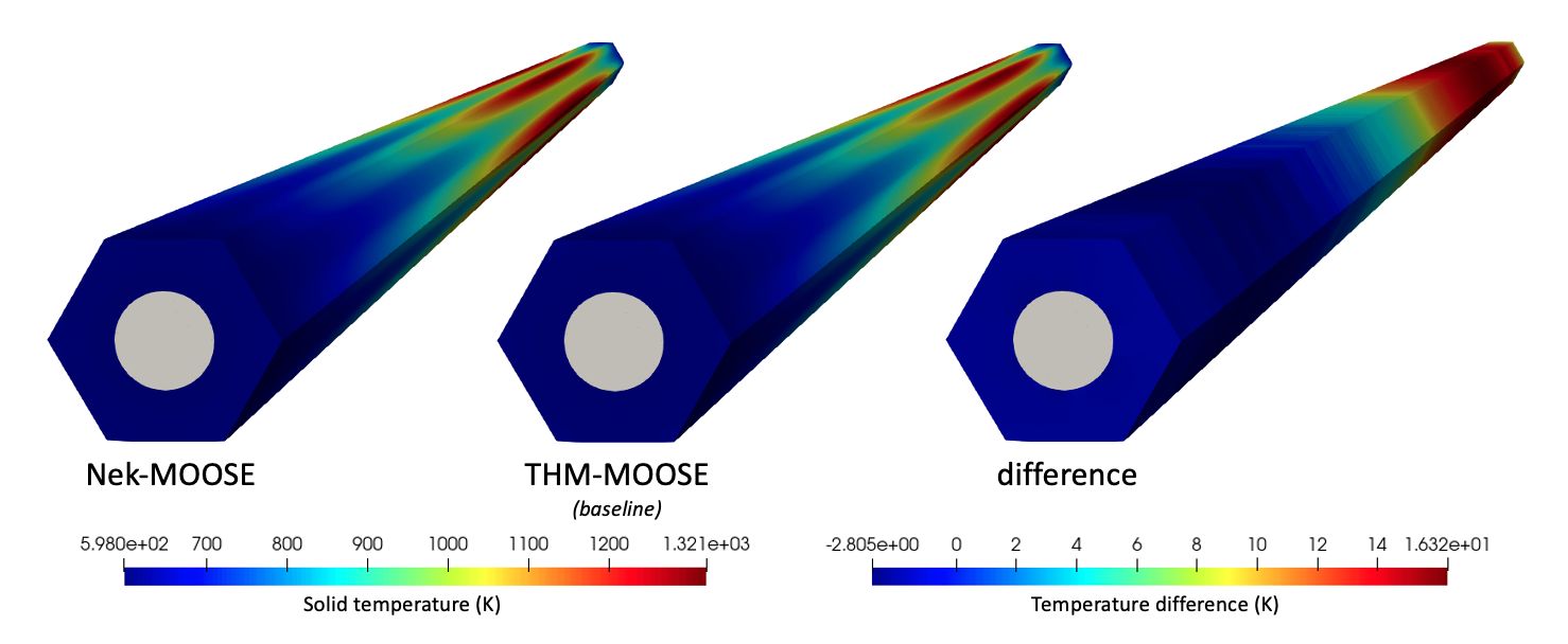
Figure 6: Solid temperature predicted for NekRS-MOOSE, baseline THM-MOOSE, and the difference between the two (NekRS minus baseline THM).
This code difference can be attributed to a number of different sources:
Because THM averages the solid heat flux along the coolant channel perimeter, THM is incapable of representing the azimuthal variation in heat flux that occurs due to the power production in the six fuel compacts.
NekRS uses a wall-resolved methodology, whereas THM uses the Dittus-Boelter correlation. Assuming the maximum temperature difference could be solely attributed to a difference in Nusselt number, a 16.3 K difference is equivalent to about a 10% difference in convective heat transfer coefficient. Errors as high as 25% may be observed when using a simple model such as the Dittus-Boelter correlation Incropera and Dewitt (2011), and a 10% difference is well within the realm of the data scatter used to originally fit the Dittus-Boelter model Winterton (1998)
Figure 7 shows the solid temperature predictions on the axial midplane for the NekRS-MOOSE, the baseline THM-MOOSE simulation, and the difference between the two (NekRS minus baseline THM). Figure 7 shows with greater clarity that the highest temperatures are observed in the fuel compacts, and that the inability of THM to resolve the angular variation in wall heat flux contributes to some spatial variation of the solid temperature difference along planes.

Figure 7: Solid temperature predicted along the axial mid-plane for NekRS-MOOSE, baseline THM-MOOSE, and the difference between the two (NekRS minus baseline THM).
Given the limitations of the 1-D area-averaged equations in THM, the temperature differences observed in Figure 6 and Figure 7 suggest that some differences between NekRS and THM could reasonably be ascribed to differences in spatial resolution and small differences in Nusselt number. A common multiscale use case of NekRS is the generation of closures for coarse-mesh thermal-fluid tools. In the next section, we will describe how Cardinal can be used to generate these heat transfer coefficients.
Heat Transfer Coefficients
In this section, we use Cardinal to correct the THM closures to better reflect the unit cell geometry and thermal-fluid conditions of interest. A correction is only computed at the single Reynolds and Prandtl numbers characterizing the unit cell ( and ). That is, a new coefficient is computed for a Dittus-Boelter type correlation with the same functional dependence on and ,
(4)
The heat transfer coefficient was defined in Eq. (3). We simply re-run the NekRS case and activate the [UserObjects] and [VectorPostprocessors] blocks (to save time, you can restart your NekRS case from one of the output files generated in the first part of this tutorial, making sure to comment out the temperature IC in the ranstube.udf because you'd now be loading temperature). Once you re-run the inputs, you will have CSV files that contain , , and in each axial layer that you can write a simple Python script to calculate and convert to a Nusselt number.
From the results of this additional simulation, Figure 8 shows the Nusselt number as a function of distance from the channel inlet computed by NekRS as a dashed line. A single average Nusselt number from the NekRS simulation is obtained as an axial average over the entire NekRS solution. Also shown for comparison is the Nusselt number predicted by the Dittus-Boelter correlation. NekRS predicts an average Nusselt number of 336.35, whereas the Dittus-Boelter correlation predicts a Nusselt number of 369.14; that is, the average NekRS Nusselt number is 8.9% smaller than the Dittus-Boelter correlation, which agrees very well with the qualitative assessment surrounding the discussion on Figure 6 that the leading contributor to a difference between the solid temperature with a NekRS fluid coupling vs. a THM fluid coupling could be ascribed to a small difference in convective heat transfer coefficient.

Figure 8: Nusselt number as a function of distance from the inlet for NekRS and the Dittus-Boelter correlation.
The NekRS simulation suggests a new coefficient for Eq. (4). The Dittus-Boelter correlation is updated in the THM input file by simply changing the 0.023 coefficient in the Nusselt number correlation to 0.021.
[Materials<<<{"href": "../syntax/Materials/index.html"}>>>]
  [Nu_mat]
    type = ADParsedMaterial<<<{"description": "Parsed expression Material.", "href": "../source/materials/ParsedMaterial.html"}>>>
    block<<<{"description": "The list of blocks (ids or names) that this object will be applied"}>>> = channel
    # Dittus-Boelter
    expression<<<{"description": "Parsed function (see FParser) expression for the parsed material"}>>> = '0.023 * pow(Re, 0.8) * pow(Pr, 0.4)'
    property_name<<<{"description": "Name of the parsed material property"}>>> = 'Nu'
    material_property_names<<<{"description": "Vector of material properties used in the parsed function"}>>> = 'Re Pr'
  []
[]Then, the THM-MOOSE simulations repeated with the NekRS-informed closure. Figure 9 compares the solid temperature between NekRS-MOOSE with the corrected THM-MOOSE simulation. With the corrected Nusselt number correlation, the maximum solid temperature difference between NekRS-MOOSE and corrected THM-MOOSE is only 10.3 K. Due to the use of an axially-constant Nusselt number in THM, a perfect agreement between NekRS-MOOSE and corrected THM-MOOSE cannot be expected. The solid temperature difference will tend to be largest in regions where the local Nusselt number (dashed red line in Figure 8) deviates most from the global average (solid red line in Figure 8). This effect is observed near the outlet of the domain, where the local Nusselt number is less than half of the average Nusselt number, causing the highest deviation between NekRS-MOOSE and corrected THM-MOOSE. On average, the magnitude of the temperature difference is only 5.3 K.
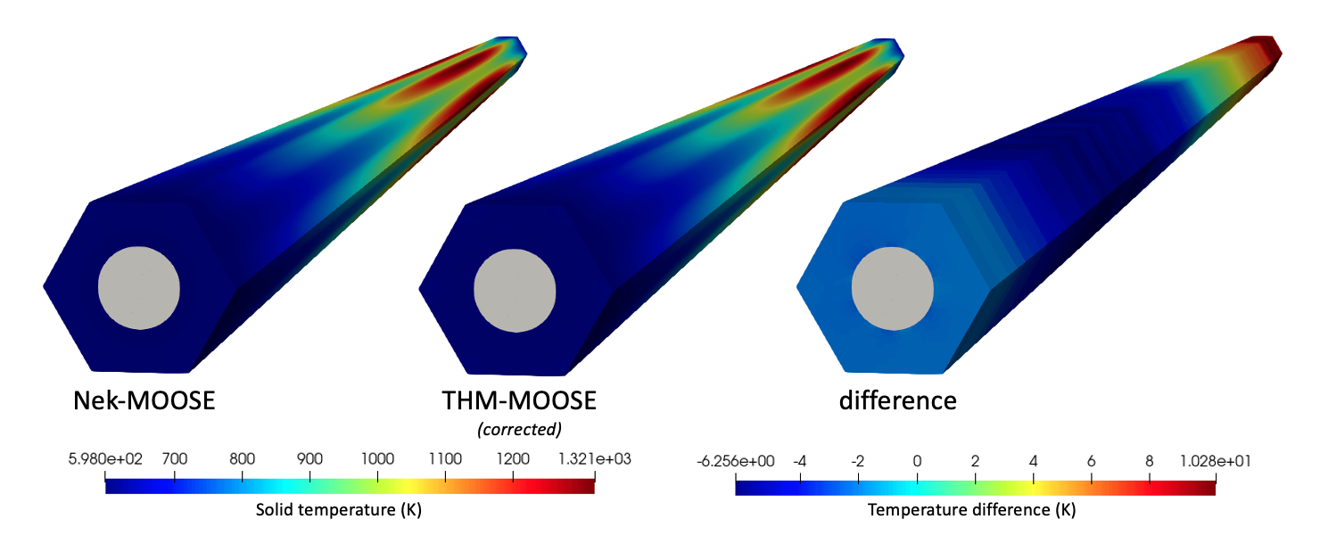
Figure 9: Solid temperature predicted for NekRS-MOOSE, corrected THM-MOOSE, and the difference between the two (NekRS minus corrected THM).
Figure 10 shows the solid temperature predictions on the axial midplane for the NekRS-MOOSE simulation, the corrected THM-MOOSE simulation, and the difference between the two (NekRS minus corrected THM). Changing the Nusselt number model in THM only affects the wall temperature applied as a boundary condition in THM; because THM solves 1-D equations, the radial variation in the error will still be present (although of a smaller magnitude due to the temperature shift induced by a change in wall temperature).
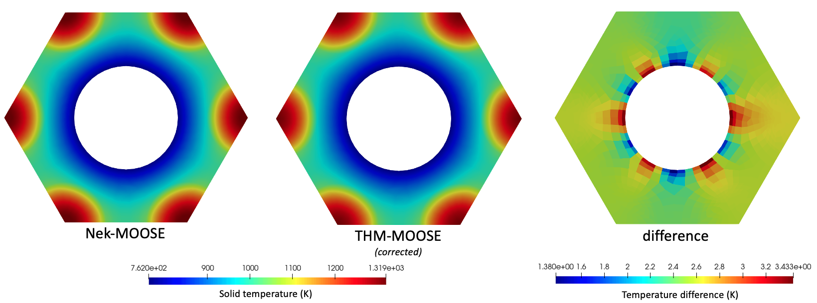
Figure 10: Solid temperature predicted along the axial midplane for NekRS-MOOSE, corrected THM-MOOSE, and the difference between the two (NekRS minus corrected THM).
Cardinal's seamless capabilities for generating coarse-mesh closures using NekRS has been demonstrated. Now, just to present a few remaining results (all obtained with the corrected THMN-MOOSE simulation). Figure 11 shows the fluid temperature predicted by NekRS-MOOSE and the corrected THM-MOOSE. Also shown for context is the solid temperature in a slice through the domain, on a different color scale than the fluid temperature. The NekRS simulation resolves the fluid thermal boundary layer, whereas the THM model uses the Dittus-Boelter correlation to represent the temperature difference between the heated wall and the bulk; therefore, the fluid temperature shown in Figure 11 for THM is the area-averaged fluid temperature. The wall temperature predicted by NekRS follows a similar distribution as the heat flux, peaking slightly downstream of the midplane due to the combined effects of convective heat transfer and the imposed sinusoidal power distribution.
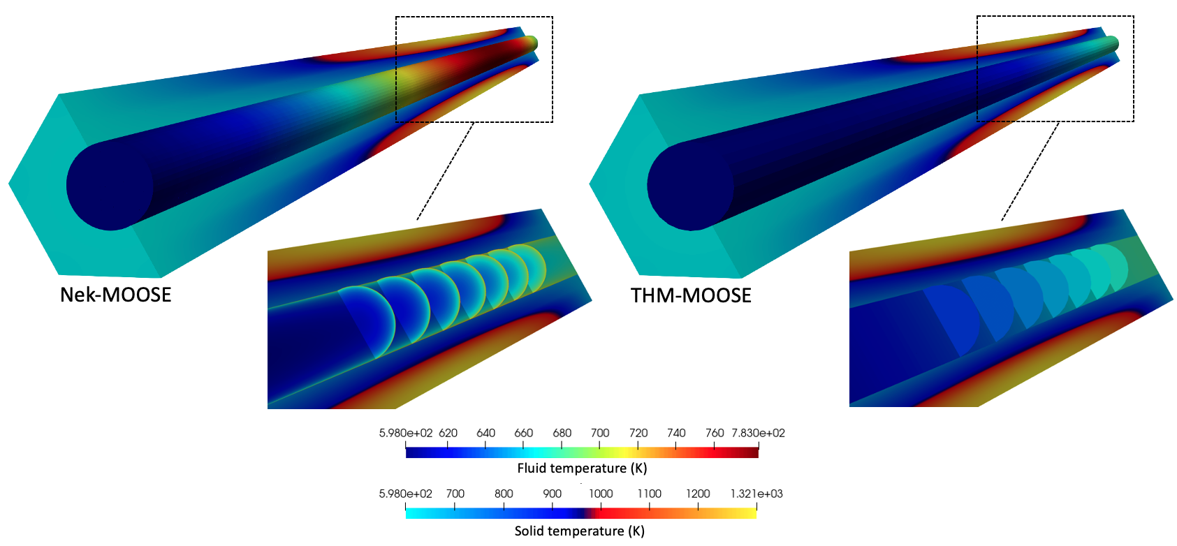
Figure 11: Fluid temperature predicted for NekRS-MOOSE and corrected THM-MOOSE.
Finally, Figure 12 compares the solutions for radially-averaged temperatures along the flow direction. As already discussed, the solid temperatures match very well between NekRS-MOOSE and THM-MOOSE and match the expected behavior for a sinusoidal power distribution. The fluid bulk temperature increases along the flow direction, with a faster rate of increase where the power density is highest.
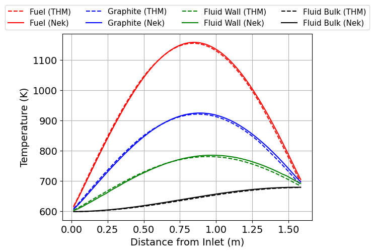
Figure 12: Radially-averaged temperatures for the NekRS-MOOSE and corrected THM-MOOSE simulations.
References
- R. A. Berry, J. W. Peterson, H. Zhang, R. C. Martineau, H. Zhao, L. Zou, and D. Andrš.
RELAP-7 Theory Manual.
Technical Report INL/EXT-14-31366, Idaho National Laboratory, 2014.[Export]
- F.P. Incropera and D.P. Dewitt.
Fundamentals of Heat and Mass Transfer, 7th ed.
John Wiley & Sons, 2011.[Export]
- INL.
High-Temperature Gas-Cooled Test Reactor Point Design.
Technical Report INL/EXT-16-38296, Idaho National Laboratory, 2016.
URL: https://tinyurl.com/v9a4hym5.[Export]
- A.J. Novak, D. Andrs, P. Shriwise, J. Fang, H. Yuan, D. Shaver, E. Merzari, P.K. Romano, and R.C. Martineau.
Coupled Monte Carlo and Thermal-Fluid Modeling of High Temperature Gas Reactors Using Cardinal.
Annals of Nuclear Energy, 177:109310, 2022.
doi:10.1016/j.anucene.2022.109310.[Export]
- R.H.S. Winterton.
Where did the Dittus and Boelter Equation Come From.
International Journal of Heat and Mass Transfer, 41:809–810, 1998.
doi:10.1016/S0017-9310(97)00177-4.[Export]