Postprocessing/Extracting the NekRS solution

Viewing the NekRS Mesh

NekRS uses a custom mesh format (with the .re2 extension). This file cannot natively be viewed in visualization software such as Paraview. Standalone NekRS users have to run at least one CFD time step, and then can only visualize the output file. This can be tedious if you need to achieve a viable CFD solve just to visualize a mesh.

Cardinal provides a way to visualize the NekRS CFD mesh. Simply set exact = true for NekRSMesh and then run in --mesh-only mode. For example, you can create a small Cardinal input file,

[Problem]
  type = NekRSStandaloneProblem
  casename = 'brick'
[]

[Mesh]
  type = NekRSMesh
  volume = true
  exact = true
[]

And then run in --mesh-only mode.

cd test/tests/nek_mesh/exact
cardinal-opt -i exact.i --mesh-only

Loading a NekRS Time History into Exodus

To access this tutorial,

cd cardinal/tutorials/load_from_exodus

For applications with "one-way" coupling of NekRS to MOOSE, you may wish to use a time history of the NekRS solution as a boundary condition/source term in another MOOSE application. For instance, for thermal striping applications, it is often a reasonable approximation to solve a NekRS CFD simulation as a standalone case, and then apply a time history of NekRS's wall temperature as a boundary condition to a solid mechanics solve. Cardinal allows you to write the NekRS solution to an Exodus file that can then be loaded to provide a time history of the CFD solution to another application. In this example, we will use the following Cardinal input file:

[Mesh]
  type = NekRSMesh
  volume = true
  order = SECOND
[]

[Problem]
  type = NekRSStandaloneProblem
  casename = 'ethier'
  output = 'temperature'
[]

[Executioner]
  type = Transient

  [TimeStepper]
    type = NekTimeStepper
  []
[]

[Outputs]
  exodus = true
[]

We incidate that we want to output the NekRS temperature onto a volume mesh mirror of second order and output to Exodus format. Then, we simply use a NekRSStandaloneProblem and NekTimeStepper to run the NekRS CFD calculation through the Cardinal wrapper. You can run this example with

mpiexec -np 4 cardinal-opt -i nek.i

which will create an output file named nek_out.e, which contains the time history of the NekRS temperature solution on the volume mesh mirror.

In order to load the entire time history of the Nek solution, we need a separate input file that will essentailly act as the surrogate for performing the Nek solution (by instead loading from the Exodus file dumped earlier). First, we use the dumped output file directly as the mesh. Because this run won't actually solve any physics (either with NekRS or with MOOSE). we next need to turn the solve off.

[Mesh]
  type = FileMesh
  file = nek_out.e
[]

[Problem]
  type = FEProblem
  solve = false
[]

Then, to load the solution from the nek_out.e, we use a SolutionUserObject. This user object will read the temp variable from the provided mesh file (which we set to our output file from the NekRS run). We omit the timestep parameter that is sometimes provided to the SolutionUserObject so that this user object will interpolate in time based on the time stepping specified in the [Executioner] block.

This user object only loads the Exodus file into a user object - to then get that solution into an AuxVariable appropriate for transferring to another application or using in other MOOSE objects, we simply convert the user object to an auxiliary variable using a SolutionAux. This will load the temp variable from the SolutionUserObject and place it into the new variable we have named nek_temp.

[UserObjects]
  [load_nek_solution]
    type = SolutionUserObject
    mesh = nek_out.e
    system_variables = 'temp'
  []
[]

[AuxVariables]
  [nek_temp]
  []
[]

[AuxKernels]
  [nek_temp]
    type = SolutionAux
    solution = load_nek_solution
    variable = nek_temp
    from_variable = temp
  []
[]

Finally, we "run" this application by specifying a Transient executioner. The time stepping scheme we specify here just indicates at which time step the data in the nek_out.e file should be interpolated to. For instance, if you ran NekRS with a time step of 1e-3 seconds, but only want to couple NekRS's temperature to a solid mechanics solve on a resolution of 1e-2 seconds, then simply set the time step size in this file to dt = 1e-2. Finally, we specify a Exodus output in this file, which you can use to see that the temperature from nek_out.e was correctly loaded (nek_temp in load_nek_out.e matches temp in nek_out.e).

[Executioner]
  type = Transient
  dt = 2e-3
  num_steps = 10
[]

[Outputs]
  exodus = true
[]

Binned Spatial Postprocessors

To access this tutorial,

cd cardinal/tutorials/subchannel

Cardinal contains features for postprocessing the NekRS solution in spatial "bins" using user objects. Available user objects include:

• NekBinnedPlaneIntegral: compute plane integrals over regions of space

• NekBinnedPlaneAverage: compute plane averages over regions of space

• NekBinnedSideIntegral: compute integrals over sidesets with subdivisions in space

• NekBinnedSideAverage: compute averages over sidesets with subdivisions in space

• NekBinnedVolumeIntegral: compute volume integrals over regions of space

• NekBinnedVolumeAverage: compute volume averages over regions of space

These user objects can be used for operations such as:

• Averaging the solution over for axisymmetric geometries

• Extracting homogenized solutions, such as for feeding volume-averaged quantities to a 3-D Pronghorn model

• Representing the solution in a different discretization form, such as a finite volume discretization of a subchannel geometry

An example of averaging over axisymmetric geometries was provided in Tutorial 1. Here, we will demonstrate averaging the NekRS solution in a fuel bundle geometry according to a subchannel discretization.

The model consists of a 7-pin Sodium Fast Reactor (SFR) fuel bundle; the mesh is shown in Figure 1. Our goal is to obtain subchannel-averaged and gap-averaged temperatures and velocities on a mesh that reflects a subchannel discretization. Note that the NekRS mesh does not have elements that align with the usual subchannel boundaries; therefore we require the ability to map the NekRS quadrature points to "bins" that represent our different regions of interest (subchannels and subchannel gaps).

Figure 1: NekRS mesh for 7-pin SFR fuel bundle; lines are shown connecting Gauss-Lobatto-Legendre (GLL) points

The NekRS input files use typical settings; the only setting of note is that for simplicity and ease of illustration, we turn the actual physics solve off by setting solver = none for the velocity and temperature in the sfr_7pin.par file.

[GENERAL]
  stopAt = numSteps
  numSteps = 1
  dt = 5.0e-4
  timeStepper = tombo2
  writeControl = steps
  writeInterval = 25
  dealiasing = yes
  polynomialOrder = 7

[VELOCITY]
  solver = none

[PRESSURE]

[TEMPERATURE]
  solver = none

Then, we specify dummy velocity, pressure, and temperature initial conditions, just for the sake of demonstrating the subchannel averaging methods.

#include "udf.hpp"

void UDF_LoadKernels(occa::properties & kernelInfo)
{
}

void UDF_Setup(nrs_t *nrs)
{
  // set initial conditions for the velocity, temperature, and pressure. Because
  // we turn off the solves, we're just doing postprocessing of whatever we set
  // for the initial conditions
  mesh_t * mesh = nrs->cds->mesh[0];

  // loop over all the GLL points and assign directly to the solution arrays by
  // indexing according to the field offset necessary to hold the data for each
  // solution component
  int n_gll_points = mesh->Np * mesh->Nelements;
  for (int n = 0; n < n_gll_points; ++n)
  {
    dfloat x = mesh->x[n];
    dfloat y = mesh->y[n];
    dfloat z = mesh->z[n];
    dfloat r = std::sqrt(x*x + y*y);

    dfloat theta;
    if (x > 0 && y >= 0)
      theta = std::atan(y / x);
    if (x < 0 && y >= 0)
      theta = M_PI - std::atan(std::abs(y / x));
    if (x < 0 && y < 0)
      theta = std::atan(y / x) + M_PI;
    if (x > 0 && y < 0)
      theta = 2 * M_PI - std::atan(std::abs(y / x));

    dfloat Vr = 0.0;
    dfloat Vt = 0.1 + 10.0 * r;
    nrs->U[n + 0 * nrs->fieldOffset] = Vr * std::cos(theta) - Vt * std::sin(theta);
    nrs->U[n + 1 * nrs->fieldOffset] = Vr * std::sin(theta) + Vt * std::cos(theta);
    nrs->U[n + 2 * nrs->fieldOffset] = 0.0;

    nrs->P[n] = x+y+z;

    nrs->cds->S[n + 0 * nrs->cds->fieldOffset[0]] = x+y+3*z;
  }
}

For instance, the temperature in the NekRS field files will remain fixed at the given function initial condition of

(1)

while the velocity is set to a swirl velocity with an angular component that increases with and zero radial component.

We will run this NekRS case with a thin wrapper input file, shown below.

[Mesh]
  type = NekRSMesh
  volume = true
[]

[Problem]
  type = NekRSStandaloneProblem
  casename = 'sfr_7pin'
  output = 'temperature velocity'
[]

[UserObjects]
  [subchannel_binning]
    type = HexagonalSubchannelBin
    bundle_pitch = 0.02583914354890463
    pin_pitch = 0.0089656996
    pin_diameter = 7.646e-3
    n_rings = 2
  []
  [subchannel_gap_binning]
    type = HexagonalSubchannelGapBin
    bundle_pitch = 0.02583914354890463
    pin_pitch = 0.0089656996
    pin_diameter = 7.646e-3
    n_rings = 2
  []
  [axial_binning]
    type = LayeredBin
    direction = z
    num_layers = 7
  []
  [average_T]
    type = NekBinnedVolumeAverage
    bins = 'subchannel_binning axial_binning'
    field = temperature
    map_space_by_qp = true
  []
  [average_T_gaps]
    type = NekBinnedPlaneAverage
    bins = 'subchannel_gap_binning axial_binning'
    field = temperature
    map_space_by_qp = true
    gap_thickness = ${fparse 0.05 * 7.646e-3}
  []
  [avg_gap_velocity]
    type = NekBinnedPlaneAverage
    bins = 'subchannel_gap_binning axial_binning'
    field = velocity_component
    velocity_component = normal
    map_space_by_qp = true
    gap_thickness = ${fparse 0.05 * 7.646e-3}
  []
[]

[AuxVariables]
  # These are just for visualizing the average velocity component with Glyphs in paraview;
  # the result of the 'avg_gap_velocity' user object will be represented as a vector "uo_" with 3 components
  [uo_x]
    family = MONOMIAL
    order = CONSTANT
  []
  [uo_y]
    family = MONOMIAL
    order = CONSTANT
  []
  [uo_z]
    family = MONOMIAL
    order = CONSTANT
  []
[]

[AuxKernels]
  [uo_x]
    type = NekSpatialBinComponentAux
    variable = uo_x
    user_object = avg_gap_velocity
    component = 0
  []
  [uo_y]
    type = NekSpatialBinComponentAux
    variable = uo_y
    user_object = avg_gap_velocity
    component = 1
  []
  [uo_z]
    type = NekSpatialBinComponentAux
    variable = uo_z
    user_object = avg_gap_velocity
    component = 2
  []
[]

[MultiApps]
  [subchannel]
    type = TransientMultiApp
    input_files = 'subchannel.i'
    execute_on = timestep_end
    sub_cycling = true
  []
  [subchannel_gap]
    type = TransientMultiApp
    input_files = 'subchannel_gap.i'
    execute_on = timestep_end
    sub_cycling = true
  []
[]

[Transfers]
  [uo_to_sub]
    type = MultiAppGeneralFieldUserObjectTransfer
    source_user_object = average_T
    to_multi_app = subchannel
    variable = average_T
  []
  [uo_to_sub2]
    type = MultiAppGeneralFieldUserObjectTransfer
    source_user_object = average_T_gaps
    to_multi_app = subchannel_gap
    variable = average_T
  []
  [uo1_to_sub]
    type = MultiAppGeneralFieldUserObjectTransfer
    source_user_object = avg_gap_velocity
    to_multi_app = subchannel_gap
    variable = avg_gap_velocity
  []
  [uox_to_sub]
    type = MultiAppGeneralFieldNearestLocationTransfer
    to_multi_app = subchannel_gap
    source_variable = uo_x
    variable = uo_x
  []
  [uoy_to_sub]
    type = MultiAppGeneralFieldNearestLocationTransfer
    to_multi_app = subchannel_gap
    source_variable = uo_y
    variable = uo_y
  []
[]

[VectorPostprocessors]
  [avg_T]
    type = SpatialUserObjectVectorPostprocessor
    userobject = average_T
  []
  [avg_T_gaps]
    type = SpatialUserObjectVectorPostprocessor
    userobject = average_T_gaps
  []
  [avg_v_gaps]
    type = SpatialUserObjectVectorPostprocessor
    userobject = avg_gap_velocity
  []
[]

[Executioner]
  type = Transient

  [TimeStepper]
    type = NekTimeStepper
  []
[]

[Outputs]
  csv = true
[]

Of note are the user objects, multiapps, and transfers. In this file, we will compute three different postprocessing operations:

• Average temperature over subchannel volumes**: We will use a user object to conduct a binned spatial average of the NekRS temperature. We first form these bins as the product of unique indices for each subchannel with unique indices for each axial layer. The HexagonalSubchannelBin object assigns a unique ID for each subchannel, for which we must provide various geometric parameters describing the fuel bundle. The LayeredBin object assigns a unique ID for equal-size layers in a given direction; here, we specify 7 axial layers. Finally, we will compute a volume average of the NekRS temperature with the NekBinnedVolumeAverage object, which constructs bins as the outer product of individual bin distributions. Because the NekRS mesh in Figure 1 has 6 elements in the axial direction, but we have specified that we want to average across 7 axial layers, we set map_space_by_qp = true. This setting will essentially apply a delta function of unity in each layer when forming the integral. Setting map_space_by_qp = false instead maps each NekRS element to a bin according to its centroid (which for this particular example would result in some of the axial bins not mapping to any elements, since the NekRS mesh is coarser than the specified number of bins).

• Average temperature over subchannel gaps**: We form the bins as the product of unique indices for each subchannel gap with unique indices for each axial layers. The HexagonalSubchannelGapBin object assigns a unique ID for each subchannel gap ID in a hexagonal fuel bundle. The LayeredBin object then assigns a unique ID for equal-size layers in the axial direction; for simplicity, we reuse the same axial binning distribution that we selected for the volume averages. Finally, we compute the planar averages of the NekRS temperature with the NekBinnedPlaneAverage object, which takes an arbitrary number of individual bin distributions (with the only requirement being that one and only one of these distribution is a "side" distribution, which for this example is the HexagonalSubchannelGapBin).

• Average the normal velocity over subchannel gaps**: We reuse the same previous bins, but set field = velocity_component for a NekBinnedPlaneAverage.

The SpatialUserObjectVectorPostprocessor outputs the bin values for the user object to the CSV format specified in the [Outputs] block. These values are ordered in the same manner that the bins are defined.

Recall that the NekRS mesh does not respect the subchannel discretization, or the desired number of axial averaging layers. Therefore, if we want to properly visualize the results of the user object, we transfer the user object to two different sub-applications which serve the sole purpose of user object visualization. We use two different sub-applications because one sub-app will use a mesh that perfectly represents the volumes of the channels, while the second sub-app will use a mesh that perfectly represents the gaps between the channels.

The application that will be used to view the volume results on the channels is shown below. This sub-application constructs a subchannel mesh with the HexagonalSubchannelMesh to receive the user object into a variable named average_T and the three components of the gap normal velocity as uo_x, uo_y, and uo_z. We set solve = false so that no physics solve occurs.

[Mesh]
  type = HexagonalSubchannelMesh
  bundle_pitch = 0.02583914354890463
  pin_pitch = 0.0089656996
  pin_diameter = 7.646e-3
  n_rings = 2
  n_axial = 7
  theta_res = 8
  height = 0.008
[]

[Problem]
  solve = false
  type = FEProblem
[]

[AuxVariables]
  [average_T]
    family = MONOMIAL
    order = CONSTANT
  []
[]

[Executioner]
  type = Transient
[]

[Outputs]
  exodus = true
[]

The application that will be used to view the gap results is shown below. This sub-application constructs a subchannel mesh with the HexagonalSubchannelGapMesh to receive the user object into a variable named average_T. We set solve = false so that no physics solve occurs.

[Mesh]
  type = HexagonalSubchannelGapMesh
  bundle_pitch = 0.02583914354890463
  pin_pitch = 0.0089656996
  pin_diameter = 7.646e-3
  n_rings = 2
  n_axial = 7
  height = 0.008
[]

[Problem]
  solve = false
  type = FEProblem
[]

[AuxVariables]
  [average_T]
    family = MONOMIAL
    order = CONSTANT
  []
  [avg_gap_velocity]
    family = MONOMIAL
    order = CONSTANT
  []

  # These are just for visualizing the average velocity component with Glyphs in paraview
  [uo_x]
    family = MONOMIAL
    order = CONSTANT
  []
  [uo_y]
    family = MONOMIAL
    order = CONSTANT
  []
  [uo_z]
    family = MONOMIAL
    order = CONSTANT
  []
[]

[Executioner]
  type = Transient
[]

[Outputs]
  exodus = true
[]

This input can be run as,

mpiexec -np 4 cardinal-opt -i nek.i

which will run with 4 MPI ranks. Because we don't specify any output block in the Nek-wrapping input file itself, the only output files are:

• nek_out_subchannel0.e, which shows the channel-averaged temperature on a subchannel discretization

• nek_out_subchannel_gap0.e, which shows the gap-averaged quantities on the gaps in a subchannel discretization

The temperature initial condition that we set from NekRS is shown in Figure 2, along with the result of the subchannel volume and gap averaging. Note that because we transferred the user object to a sub-application with a mesh that respects our axial bins, we perfectly represent the channel-wise average temperatures.

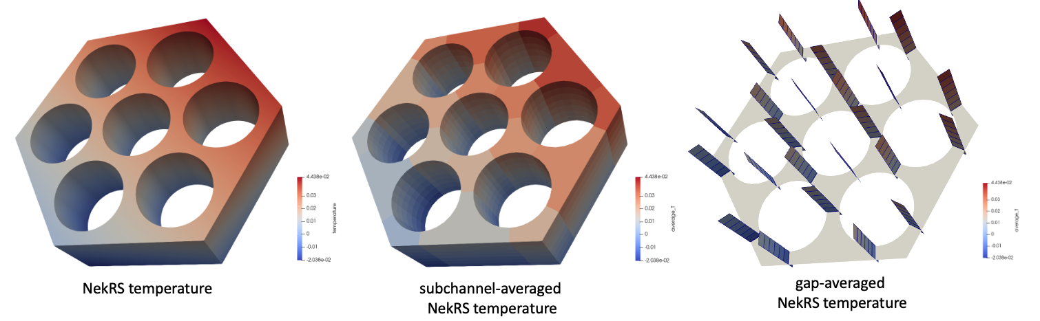
Figure 2: NekRS temperature (left), subchannel-averaged temperature (middle), and gap-averaged temperature (right) computed using Cardinal user objects

By applying the "glyph" filter in Paraview, we can visualize the gap-normal velocity with arrows. Otherwise, the result of the avg_gap_velocity user object is a magnitude, which would need to be combined with the gap unit normals (defined in the HexagonalSubchannelGapBin documentation) to visualize the direction.

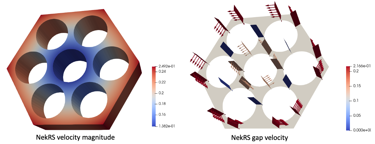
Figure 3: NekRS temperature (left), subchannel-averaged temperature (middle), and gap-averaged temperature (right) computed using Cardinal user objects

For other geometries, other binning strategies can be used. Available user objects for specifying spatial bins are:

• HexagonalSubchannelGapBin

• HexagonalSubchannelBin

• LayeredBin

• LayeredGapBin

• RadialBin

For example, you can compute an average over a number of planes perpendicular to the axis, split into two layers, by combining the two bin user objects shown below.

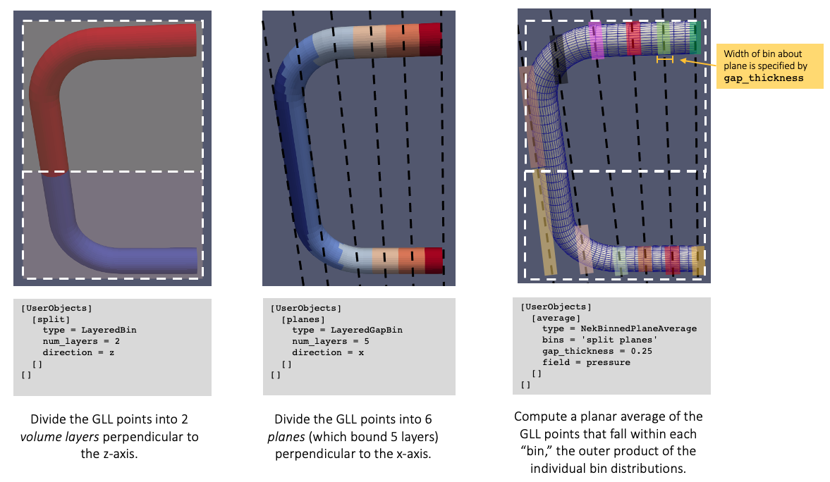
Figure 4: Example use case for arbitrary combinations of bin objects for spatial postprocessing of NekRS solutions