Running NekRS as a Standalone Application

Standalone Simulations

As part of Cardinal's build process, the nekrs executable used to run standalone NekRS cases is compiled and placed in the $NEKRS_HOME/bin directory. This directory also contains other scripts used to simplify the use of the nekrs executable. To use these scripts to run standalone NekRS cases, we recommend adding this location to your path:

export PATH=$NEKRS_HOME/bin:$PATH

Then, you can run any standalone NekRS case simply by having built Cardinal - no need to separately build and compile NekRS. For instance, try running the ethier example that ships with NekRS:

cd contrib/nekRS/examples/ethier
nrsmpi ethier 4

And that's it! No need to separately compile NekRS.

Thinly-Wrapped Simulations

To access this tutorial:

cd cardinal/tutorials/standalone

To contrast with the previous example, you can achieve the same "standalone" calculations via Cardinal, which you might be interested in to leverage Cardinal's postprocessing and data I/O features. Some useful features include:

• Postprocessors to evaluate max/mins, area/volume integrals and averages, and mass flux-weighted side integrals of the NekRS solution

• Extracting the NekRS solution into any output format supported by MOOSE (such as Exodus and VTK - see the full list of formats here).

Instead of running a NekRS input with the nekrs executable, you can instead create a "thin" wrapper input file that runs NekRS as a MOOSE application (but allowing usage of the postprocessing and data I/O features of Cardinal). For wrapped applications, NekRS will continue to write its own field file output during the simulation as specified by settings in the .par file.

To run NekRS via MOOSE, without any physics coupling, Cardinal simply replaces calls to MOOSE solve methods with NekRS solve methods available through an Application Programming Interface (API). There are no data transfers to/from NekRS. A thinly-wrapped simulation uses:

1. NekRSMesh: create a "mirror" of the NekRS mesh, which can optionally be used to interpolate a high-order NekRS solution into a lower-order mesh (in any MOOSE-supported format).

2. NekRSStandaloneProblem: allow MOOSE to run NekRS

For this tutorial, we will use the turbPipe example that ships with the NekRS repository as an example case. This case models turbulent flow in a cylindrical pipe (cast in non-dimensional form). The domain consists of a pipe of diameter 1 and length 20 with flow in the direction. The NekRS mesh is shown in Figure 1. Note that the visualization of NekRS's mesh in Paraview draws lines connecting the GLL points, and not the actual element edges.

Figure 1: NekRS mesh, with lines connecting GLL points and sideset IDs.

The NekRS input files are exactly the same that would be used to run this model as a standalone case. These input files include:

• turbPipe.re2: NekRS mesh

• turbPipe.par: High-level settings for the solver, boundary condition mappings to sidesets, and the equations to solve

• turbPipe.udf: User-defined C++ functions for on-line postprocessing and model setup

• turbPipe.oudf: User-defined Open Concurrent Compute Abstraction (OCCA) kernels for boundary conditions and source terms

This particular input also uses an optional turbPipe.usr file for setting up other parts of the model using the Nek5000 backend. We refer a discussion of these files to the NekRS documentation website.

Instead of running this input directly with the NekRS scripts like we did in Standalone Simulations , we instead wrap the NekRS simulation as a MOOSE application. The Cardinal input file is shown below; this is not the simplest file that we need to run NekRS, but we add extra features to be described shortly.

[Mesh]
  type = NekRSMesh
  volume = true
  order = SECOND
[]

[Problem]
  type = NekRSStandaloneProblem
  casename = 'turbPipe'
  output = 'pressure velocity'
[]

[Postprocessors]
  [outlet_p]
    type = NekSideAverage
    boundary = '2'
    field = pressure
  []
  [inlet_p]
    type = NekSideAverage
    boundary = '1'
    field = pressure
  []
  [mdot]
    type = NekMassFluxWeightedSideIntegral
    boundary = '1'
    field = unity
  []

  # subtracts the two pressure postprocessors
  [dP]
    type = DifferencePostprocessor
    value1 = outlet_p
    value2 = inlet_p
  []
[]

[UserObjects]
  [axial_bins]
    type = LayeredBin
    direction = z
    num_layers = 20
  []
  [radial_bins]
    type = RadialBin
    vertical_axis = z
    rmax = 0.5
    nr = 12
    growth_r = 0.9
  []
  [volume_averages]
    type = NekBinnedVolumeAverage
    bins = 'radial_bins axial_bins'
    field = velocity_z
    map_space_by_qp = true
  []
[]

[AuxVariables]
  [volume_averages]
    family = MONOMIAL
    order = CONSTANT
  []
[]

[AuxKernels]
  [volume_averages]
    type = SpatialUserObjectAux
    variable = volume_averages
    user_object = volume_averages
  []
[]

[MultiApps]
  [sub]
    type = TransientMultiApp
    input_files = sub.i
    execute_on = timestep_end
  []
[]

[Transfers]
  [uo_to_sub]
    type = MultiAppGeneralFieldUserObjectTransfer
    to_multi_app = sub
    source_user_object = volume_averages
    variable = avg_velocity
  []
[]

[Executioner]
  type = Transient

  [TimeStepper]
    type = NekTimeStepper
  []
[]

[Outputs]
  exodus = true
  csv = true

  # this hides these values from the screen for neater output
  hide = 'outlet_p inlet_p'
[]

The essential blocks in the input file are:

• Mesh: creates a lower-order mirror of the NekRS mesh

• Problem: replaces MOOSE finite element solves with NekRS solves

• Executioner: controls the time stepping according to the settings in the NekRS input files

• Outputs: outputs any results that have been projected onto the NekRSMesh to the specified format.

This input file is run with:

mpiexec -np 4 cardinal-opt -i nek.i

which will run with 4 MPI ranks. This will create a number of output files:

• nek_out.e shows the NekRS solution mapped to a MOOSE mesh

• nek_out_sub0. shows the result of a postprocessing operation, mapped to a different MOOSE mesh

• nek_out.csv shows the CSV postprocessor values

• turbPipe0.f<n> are the NekRS output files, where <n> is an integer representing output step index in NekRS

When running this tutorial, the NekRS output file is the nek_out.e file, while the output of the sub-application is the nek_out_sub0.e file.

Now that you know how to run, let's describe the rest of the contents in the nek.i input file. This file adds a few additional postprocessing operations to compute:

• pressure drop, computed by subtracting the inlet average pressure from the outlet average pressure with two NekSideAverage postprocessors and the DifferencePostprocessor

• mass flowrate, computed with a NekMassFluxWeightedSideIntegral postprocessor

[Postprocessors]
  [outlet_p]
    type = NekSideAverage
    boundary = '2'
    field = pressure
  []
  [inlet_p]
    type = NekSideAverage
    boundary = '1'
    field = pressure
  []
  [mdot]
    type = NekMassFluxWeightedSideIntegral
    boundary = '1'
    field = unity
  []

  # subtracts the two pressure postprocessors
  [dP]
    type = DifferencePostprocessor
    value1 = outlet_p
    value2 = inlet_p
  []
[]

This will print to the screen for each time step the values of these postprocessors, which can be useful for evaluating solution progression:

+----------------+----------------+----------------+
| time           | dP             | mdot           |
+----------------+----------------+----------------+
|   0.000000e+00 |   0.000000e+00 |   0.000000e+00 |
|   6.000000e-03 |  -3.334281e+02 |  -7.854005e-01 |
|   1.200000e-02 |   1.637766e+02 |  -7.853985e-01 |
|   1.800000e-02 |   1.540674e+00 |  -7.853985e-01 |
+----------------+----------------+----------------+

By setting csv = true in the output block, we will also write these postprocessors into a CSV format, which is convenient for script-based postprocessing operations:

time,dP,mdot
0,0,0
0.006,-333.42814336273,-0.78540045786239
0.012,163.77659967808,-0.78539846245391
0.018,1.540674311383,-0.78539846245391

By setting output = 'pressure velocity' for NekRSStandaloneProblem, we interpolate the NekRS solution (which for this example has degrees of freedom per element, since polynomialOrder = 7 in turbPipe.par) onto a second-order version of the same mesh by creating MooseVariables named P and velocity. You can then apply any MOOSE object to those variables, such as postprocessors, userobjects, auxiliary kernels, and so on. You can also transfer these variables to another MOOSE application if you want to couple NekRS to MOOSE without feedback - such as for using Nek's velocity to transport a passive scalar in another MOOSE application.

The axial velocity computed by NekRS, as well as the velocity interpolated onto the mesh mirror, are shown in Figure 2.

Figure 2: NekRS computed axial velocity (top) and the velocity interpolated onto the NekRSMesh mirror (bottom)

We can also apply several userobjects directly to the NekRS solution for a number of postprocessing operations. Below, we perform a volume average of in 12 radial bins discretized into 20 axial layers.

[UserObjects]
  [axial_bins]
    type = LayeredBin
    direction = z
    num_layers = 20
  []
  [radial_bins]
    type = RadialBin
    vertical_axis = z
    rmax = 0.5
    nr = 12
    growth_r = 0.9
  []
  [volume_averages]
    type = NekBinnedVolumeAverage
    bins = 'radial_bins axial_bins'
    field = velocity_z
    map_space_by_qp = true
  []
[]

If we want to view the output of this averaging on the NekRSMesh, we could visualize it with a SpatialUserObjectAux.

[AuxVariables]
  [volume_averages]
    family = MONOMIAL
    order = CONSTANT
  []
[]

[AuxKernels]
  [volume_averages]
    type = SpatialUserObjectAux
    variable = volume_averages
    user_object = volume_averages
  []
[]

The result of the volume averaging operation is shown in Figure 3. Because the NekRS mesh elements don't fall nicely into the specified bins, we actually can only see the bin averages that the mesh mirror elements "hit" (according to their centroid). This is obviously non-ideal because the underlying form of the NekRS mesh is distorting the visualization of the volume average (even though the NekRS mesh element layout doesn't affect the actual averaging and the userobject stores the values of all 12 radial bins, even if they can't be seen).

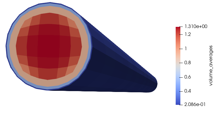
Figure 3: Representation of the volume_averages binned averaging on the NekRS mesh mirror

Instead, we can leverage MOOSE's MultiApp system to transfer the user object to a sub-application with a different mesh than what is used in NekRS. Then we can visualize the averaging operation perfectly without concern for the fact that the NekRS mesh doesn't have elements that fall nicely into the 12 radial bins. To do this, we create a sub-application with mesh elements exactly matching the user object binning and turn the solve off by setting solve = false, so that this input file only serves to receive data onto a different mesh.

[Mesh]
  [disc]
    type = AnnularMeshGenerator
    rmax = 0.5
    rmin = 0.0
    nr = 12
    nt = 24
    growth_r = 0.9
  []
  [extrude]
    type = AdvancedExtruderGenerator
    input = disc
    heights = '20.0'
    num_layers = '20'
    direction = '0 0 1'
  []
[]

[Problem]
  solve = false
  type = FEProblem
[]

[AuxVariables]
  [avg_velocity]
    family = MONOMIAL
    order = CONSTANT
  []
[]

[Executioner]
  type = Transient
[]

[Outputs]
  exodus = true
[]

Then we transfer the volume_averages user object to the sub-application.

[MultiApps]
  [sub]
    type = TransientMultiApp
    input_files = sub.i
    execute_on = timestep_end
  []
[]

[Transfers]
  [uo_to_sub]
    type = MultiAppGeneralFieldUserObjectTransfer
    to_multi_app = sub
    source_user_object = volume_averages
    variable = avg_velocity
  []
[]

The user object received on the sub-application is shown in Figure 4, which exactly represents the 12 radial averaging bins.

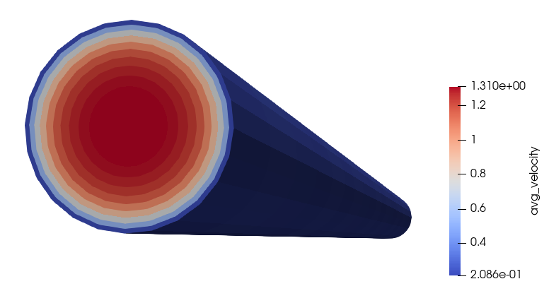
Figure 4: Representation of the volume_averages binned exactly as computed by user object