LWR Pincell with OpenMC's Random Ray Solver
In this tutorial, you will learn:
How to convert a continuous energy Monte Carlo model to a multi-group The Random Ray Method (TRRM) model
How to couple OpenMC's TRRM solver to MOOSE with a fission heat source and temperature feedback
The advantages and disadvantages of TRRM compared to continuous energy Monte Carlo
While this tutorial does not apply density feedback for simplicity, this capability is supported when running the TRRM solver and has been verified with the Doppler slab benchmark.
To access this tutorial,
cd cardinal/tutorials/rr_lwr_pincell
Geometry and Computational Models
This model consists of a single UO2 pincell from a continuous energy version of the 3D C5G7 benchmark in Smith et al. (2006). Instead of using the multi-group cross sections from the C5G7 benchmark specifications, the material properties in Cathalau et al. (1996) are used to demonstrate conversion from a continuous energy model to a multi-group TRRM model. The pincell consists of a UO2 fuel pellet clad with Zr. The pin is surrounded by borated water, and there is a He gap between the fuel and cladding. The relevant dimensions of the problem can be found in Table 1.
Table 1: Geometric specifications for the LWR pincell
| Parameter | Value (cm) |
|---|---|
| Fuel pellet outer radius | 0.4095 |
| Fuel clad inner radius | 0.418 |
| Fuel clad outer radius | 0.475 |
| Pin pitch | 1.26 |
| Fuel height | 200 |
A total core power of 3000 MWth is assumed to be uniformly distributed among 273 rodded fuel assemblies, each with 264 pins (which do not have a uniform power distribution due to the control rods and guide tubes). The tallies added by Cardinal will therefore be normalized according to the per-pin power:
(1)
where is the number of fuel assemblies in the core and is the number of pins per assembly. This tutorial considers heat conduction within the fuel and the cladding, but does not model heat transport in the coolant. Instead, a convective heat flux boundary condition ( W m K) with the following fluid temperature
(2)
is applied to the outer surface of the cladding. Although simplistic, this lets us focus this tutorial on TRRM and its unique features, while removing some complexity of including a fluids solver (which you can extend should it be desired). The common parameters for the model can be found in common.i:
# Some properties that can be modified to change the model.
## The radius of a fuel pin (cm).
R_FUEL = 0.4095

## The thickness of the fuel-clad gap (cm).
T_F_C_GAP = 0.0085

## The thickness of the Zr fuel pin cladding (cm).
T_ZR_CLAD = 0.057

## The pitch of a single lattice element (cm).
PITCH = 1.26

## The height of the fuel pin (cm). The pin geometry will range from -HEIGHT/2 to HEIGHT/2
HEIGHT = 200.0

## The number of axial layers in the multiphysics model.
AXIAL_LAYERS = 100

## The power of the pincell (W). Equal to 3000e6 / (273 * 264)
P_PIN = 41625.0

## The inlet and outlet temperature of the coolant, alongside the average of the
## inlet/outlet temperature (K).
T_INLET  = 573.0
T_OUTLET = 623.0
T_AVG    = 598

## The convective heat transfer coefficient (W/m2/K)
CONV_HT_COEFF = 1000.0

## Thermal conductivity of the fuel, cladding, and gap (W/m/K).
K_FUEL = 5.0
K_CLAD = 50.0
K_GAS = 1.0Continuous Energy OpenMC Model
OpenMC's Python API is used to generate the CSG model for this LWR pincell. We begin by defining a helper function, build_sr_pin, which we will use to subdivide the CSG region representing the UO2 pellet portion of the pincell. This serves two purposes: i) to improve the resolution of the temperature feedback sent to OpenMC, and ii) to apply spatial discretization for TRRM. The function subdivides the radial dimension of a cylindrical region with equal-volume subdivisions, and the azimuthal dimension is discretized uniformly.
def build_sr_pin(pin_fill, num_rings, num_sectors, fuel_or_surf) -> openmc.Universe:
  avg_volume = np.pi * (fuel_or_surf.r**2) / num_rings
  radii = np.zeros(num_rings + 1)
  angles = [2 * j * openmc.pi / num_sectors for j in range(num_sectors)]
  radii[0] = 0.0

  # Calculate radii for equal-volume fuel rings.
  for i in range(1, num_rings + 1):
    radii[i] = np.sqrt(radii[i-1]**2 + avg_volume / np.pi)

  print('Equal volume slices:', avg_volume)
  print('Fuel radii:', radii)

  radial_surf = [openmc.ZCylinder(x0=0, y0=0, r=surf_r) for surf_r in radii[1:-1]]
  radial_surf.append(fuel_or_surf)
  azimuthal_surf = [openmc.Plane(a=-openmc.sin(angle), b=openmc.cos(angle), c=0, d=0) for angle in angles]

  pincell_base = openmc.Universe()
  cell_id = 0

  for i in range(num_rings):
    r_region = -radial_surf[i]
    if i > 0:
      r_region &= +radial_surf[i - 1]

    if num_sectors < 2:
      # If there are no azimuthal segments, just divide in r.
      cell = openmc.Cell(fill=pin_fill, region=r_region, name=f'Fuel cell {cell_id}')
      pincell_base.add_cell(cell)
      cell_id += 1
    else:
      # In the case where there are multiple azimuthal segments, we subdivide in r and theta.
      for j in range(num_sectors):
        azimuthal_region = +azimuthal_surf[j] & -azimuthal_surf[(j+1) % num_sectors]
        cell = openmc.Cell(fill=pin_fill, region=r_region & azimuthal_region, name=f'Fuel cell {cell_id}')
        pincell_base.add_cell(cell)
        cell_id += 1
  return pincell_base
Afterwards, we define continuous energy material properties for the UO2 fuel (uo2), Zr cladding (zr), and borated water coolant (h2o). Once materials are defined, we create the surfaces and cells necessary to build the full pincell with CSG in the radial plane. build_sr_pin is then used to create a universe which is populated with the discretized pincell. In this problem the azimuthal dimension of the fuel pin itself is symmetric, so we simply subdivide the fuel into 3 radial regions. The radial geometry is then added to a lattice to extrude it into 100 layers axially. The lattice is placed in a cell which applies vacuum boundary conditions on the top and bottom of the pincell, while reflective boundary conditions are applied on the remaining sides of the geometry. Finally, we add the materials and geometry to a model container and set some simulation settings for the continuous energy model. The radial discretization of the OpenMC CSG geometry can be found in Figure 1.
For most continuous-energy simulations model.materials does not need to be set prior to writing the model.xml file to disk with model.export_to_model_xml(). However, when using model.convert_to_multigroup(), model.materials must be set as the conversion function does not attempt to discover materials from the geometry.
  ## Fuel region: UO2 at ~1% enriched.
  uo2_comp = 1.0e24 * np.array([8.65e-4, 2.225e-2, 4.622e-2])
  uo2_frac = uo2_comp / np.sum(uo2_comp)
  uo2 = openmc.Material(name = 'UO2 Fuel')
  uo2.add_nuclide('U235', uo2_frac[0], percent_type = 'ao')
  uo2.add_nuclide('U238', uo2_frac[1], percent_type = 'ao')
  uo2.add_element('O', uo2_frac[2], percent_type = 'ao')
  uo2.set_density('atom/cm3', np.sum(uo2_comp))

  ## Cladding, pure Zr metal.
  zr = openmc.Material(name = 'Zr Cladding')
  zr.add_element('Zr', 1.0, percent_type = 'ao')
  zr.set_density('atom/cm3', 1.0e24 * 4.30e-2)

  ## Moderator and coolant, boronated water.
  h2o_comp = 3.0e24 * np.array([3.35e-2, 2.78e-5])
  h2o_frac = h2o_comp / np.sum(h2o_comp)
  h2o = openmc.Material(name = 'H2O Moderator')
  h2o.add_element('H', 2.0 * h2o_frac[0], percent_type = 'ao')
  h2o.add_element('O', h2o_frac[0], percent_type = 'ao')
  h2o.add_element('B', h2o_frac[1], percent_type = 'ao')
  h2o.set_density('atom/cm3', np.sum(h2o_comp))
  h2o.add_s_alpha_beta('c_H_in_H2O')

  # Build the pincell geometry.
  # Some useful surfaces.
  fuel_pin_or = openmc.ZCylinder(r = specs.R_FUEL)
  fuel_gap_or = openmc.ZCylinder(r = specs.R_FUEL + specs.T_F_C_GAP)
  fuel_zr_or = openmc.ZCylinder(r = specs.R_FUEL + specs.T_F_C_GAP + specs.T_ZR_CLAD)
  fuel_bb = openmc.model.RectangularPrism(width = specs.PITCH, height = specs.PITCH, boundary_type = 'reflective')
  pin_bot = openmc.ZPlane(z0 = -0.5 * specs.HEIGHT, boundary_type = 'vacuum')
  pin_top = openmc.ZPlane(z0 = 0.5 * specs.HEIGHT, boundary_type = 'vacuum')

  ## Create cells for the cladding, gap, and water.
  ## The total cross section of the He gap hits the void guard in the random ray solver. We
  ## model it as void to avoid numerical instabilities.
  gap_cell = openmc.Cell(fill = None, region = +fuel_pin_or & -fuel_gap_or, name = 'Gap Cell')
  clad_cell = openmc.Cell(fill = zr, region = +fuel_gap_or & -fuel_zr_or, name = 'Clad Cell')
  mod_cell = openmc.Cell(fill = h2o, region = +fuel_zr_or, name = 'Moderator Cell')

  ## Use the helper function to build a universe filled with subdivided
  ## fuel source regions. The fuel pin is symmetric in the azimuthal plane, so we only need
  ## to subdivide the pin radially.
  fuel_pin_uni = build_sr_pin(uo2, 3, 1, fuel_pin_or)
  ## Add the other cells to this universe.
  fuel_pin_uni.add_cells([gap_cell, clad_cell, mod_cell])

  ## Place the pin in a lattice for more efficient transport.
  one_d_lattice = openmc.RectLattice(name = 'Lattice')
  one_d_lattice.pitch = (specs.PITCH, specs.PITCH, specs.HEIGHT / specs.AXIAL_LAYERS)
  one_d_lattice.lower_left = (-0.5 * specs.PITCH, -0.5 * specs.PITCH, -0.5 * specs.HEIGHT)
  one_d_lattice.universes = [[[fuel_pin_uni]]] * specs.AXIAL_LAYERS
  lattice_cell = openmc.Cell(fill = one_d_lattice, region = -fuel_bb & +pin_bot & -pin_top)
  root_uni = openmc.Universe(cells=[lattice_cell])

  # The model container.
  ce_model = openmc.Model()
  ce_model.materials = openmc.Materials([uo2, zr, h2o])
  ce_model.geometry = openmc.Geometry(root=root_uni)
  src_ll = (-0.5 * specs.PITCH, -0.5 * specs.PITCH, -0.5 * specs.HEIGHT)
  src_ur = ( 0.5 * specs.PITCH,  0.5 * specs.PITCH,  0.5 * specs.HEIGHT)

  # Simulation settings.
  ce_model.settings.source.append(openmc.IndependentSource(space = openmc.stats.Box(lower_left = src_ll, upper_right = src_ur)))
  ce_model.settings.batches = 100
  ce_model.settings.inactive = 10
  ce_model.settings.particles = 1000
  ce_model.settings.temperature['method'] = 'interpolation'
  ce_model.settings.temperature['tolerance'] = 5000.0
  ce_model.settings.temperature['range'] = (294.0, 3000.0)
  ce_model.settings.temperature['multipole'] = True
  ce_model.settings.temperature['default'] = 0.5 * (573.0 + 623.0)
 model.](../media/rr_openmc_cells.png)
Figure 1: Radial source region discretization used by the TRRM model.
Converting to a Random Ray Model
Converting the continuous energy model into a multi-group TRRM model is streamlined by the autoconversion utilities provided by OpenMC. We create a copy of the continuous energy model with rr_model = copy.deepcopy(ce_model) (to avoid overwriting the continuous energy model) and then call rr_model.convert_to_multigroup(...) followed by rr_model.convert_to_random_ray(...).
  rr_model = copy.deepcopy(ce_model)
  rr_model.convert_to_multigroup(
    method="material_wise",
    groups='CASMO-2',
    nparticles=5000,
    overwrite_mgxs_library=False,
    mgxs_path="mgxs.h5",
    correction="P0",
    temperatures = [294, 600, 900, 1200, 1500, 1800, 2100, 2400]
  )
  rr_model.convert_to_random_ray()
rr_model.convert_to_multigroup(...) runs a series of OpenMC continuous energy calculations to generate MGXS. We choose the material_wise option, which runs the provided model (with no modifications) to generate MGXS for each material. This is the highest fidelity option provided by the autoconversion function, taking into account both self-shielding and element-shielding effects. Additionally, material_wise is the only option which supports the generation of MGXS for k-eigenvalue problems (the other options run fixed source calculations). We select the CASMO-2 group structure for the energy discretization to reduce the runtime of this tutorial. This is a fairly coarse group structure; we recommend using more energy groups to minimize bias in power distributions and integral quantities as two groups will not be sufficient for most problems (without the use of transport equivalences). Finally, we specify a list of temperatures to use when generating MGXS. convert_to_multigroup will run a continuous energy OpenMC simulation for each provided temperature where every material in the model is set to that temperature (isothermal conditions). This proves to be a severe approximation for multiphysics calculations where large temperature differences exist between different materials, such as LWR problems (where the coolant has a temperature of ~600 K and the fuel has a temperature of ~1400 K). We chose to use isothermal conditions in this tutorial to simplify the generation of MGXS - care should be exercised if using this option for production calculations. We recommend reading the OpenMC user guide for generating MGXS to review the pros and cons of the autoconvert function and to learn how you can generate the MGXS without relying on the autoconvert function. A final choice that we make for MGXS generation is the scattering treatment - we select a P0 transport correction (correction="P0") to minimize bias introduced in the scattering source. This is often sufficient for LWR applications.
Converting to a random ray model requires minimal user knowledge. OpenMC will examine the bounding box of our pincell to determine the maximum chord length, and set the inactive length to that distance. The maximum chord length is often larger than ten mean free paths in reactor applications, and so ray initialization bias is wiped away with this choice. The active distance is set to five times the maximum chord length. The inactive and active ray lengths can be set to different values if they are found to be insufficient. This function also sets the ray source to the geometric bounding box, and takes a guess as to how many rays will be required. The number of rays should be set by the user as the default guess is almost never sufficient.
After converting to a TRRM model, we set some discretization parameters specific to our problem. This includes further source region subdivision of the coolant region using a uniform mesh (known as cell-under-voxel source region decomposition). This discretization is easy to apply, however it can yield very small source regions near the intersection of the boundaries of a mesh voxel and a CSG cell (which is less likely to get hit by a ray). This may result in stability issues in some cases and worse statistics for tallies. An additional disadvantage of this subdivision approach is that Cardinal cannot map to these regions as they are created on the fly during the simulation process; we recommend manual subdivision for most multiphysics simulations unless the regions do not require mapped tallies or temperature/density feedback. We also set the source region discretization to either: i) flat sources, or ii) linear sources (depending on command line arguments provided to the Python script). Linear sources will result in an increase in accuracy for a given geometric discretization at the cost of increased computational time, and potentially introducing negative source values (which OpenMC will set to zero). These negative values are a symptom of a very coarse source region discretization. Finally, we set random_ray['diagonal_stabilization_rho'] = 1.0 to ensure our use of a transport correction doesn't destabilize the combined scattering source/power iteration used by TRRM.
  ## Create a mesh to do cell-under-voxel decomposition of the moderator
  sr_depth_voxels = 10
  sr_mesh = openmc.RegularMesh().from_domain(rr_model.geometry)
  sr_mesh.dimension = (sr_depth_voxels, sr_depth_voxels, 1)
  ## Apply the source region mesh.
  rr_model.settings.random_ray['source_region_meshes'] = [(sr_mesh, [mod_cell])]

  ## Set the source region type and the transport stabilization.
  rr_model.settings.random_ray['diagonal_stabilization_rho'] = 1.0
  if use_linear_source:
    rr_model.settings.random_ray['source_shape'] = 'linear'
    print('- Using linear source regions')
  else:
    rr_model.settings.random_ray['source_shape'] = 'flat'
    print('- Using flat source regions')

  ## Write the final random ray model.
  rr_model.export_to_model_xml()
The flat source random ray model can be generated with,
python make_openmc_model.py -r
and the linear source model can be generated with,
python make_openmc_model.py -r --linear
MOOSE Heat Conduction Model
The MOOSE heat transfer module is used to solve for steady-state heat conduction,
(3)
where is the solid thermal conductivity, is the solid temperature, and is a volumetric heat source in the solid.
Because heat transfer and fluid flow in the borated water is not modeled in this example, heat removal by the fluid is approximated by setting the outer surface of the cladding to a convection boundary condition,
(4)
where and are described in the model parameters.
The gap region is unmeshed, and a quadrature-based thermal contact model is applied based on the sum of thermal conduction and thermal radiation (across a transparent medium). For a paired set of boundaries, each quadrature point on boundary is paired with the nearest quadrature point on boundary . Then, the sum of the radiation and conduction heat fluxes imposed between quadrature point pairs is
(5)
where is the Stefan-Boltzmann constant, is the temperature at a quadrature point, is the temperature of the nearest quadrature point across the gap, and are emissivities of boundaries and , respectively, and is the conduction resistance. For cylindrical geometries, the conduction resistance is given as
(6)
where are the radial coordinates associated with the outer and inner radii of the cylindrical annulus, is the height of the annulus, and is the thermal conductivity of the annulus material.
Multiphysics Coupling
Mesh
In this multiphysics model, the heat conduction and neutronics solves use the same mesh. This is generated with a standalone input file (solid_mesh.i):
!include common.i

[Mesh]
  [Pincell]
    type = PolygonConcentricCircleMeshGenerator
    num_sides = 4
    num_sectors_per_side = '4 4 4 4'
    ring_radii = '0.23642494 0.33435535 ${R_FUEL}
                  ${fparse R_FUEL + T_F_C_GAP}
                  ${fparse R_FUEL + T_F_C_GAP + T_ZR_CLAD}'
    ring_intervals = '1 1 1 1 1'
    polygon_size = ${fparse 0.5 * PITCH}

    ring_block_ids = '0 1 1
                      2
                      3'
    ring_block_names = 'uo2_tri uo2 uo2
                        gap
                        clad'
    background_block_ids = '4'
    background_block_names = 'water'
    background_intervals = 1

    flat_side_up = true
    quad_center_elements = false

    create_outward_interface_boundaries = false
  []
  [3D_Core]
    type = AdvancedExtruderGenerator
    input = 'Pincell'
    heights = '${HEIGHT}'
    num_layers = '${AXIAL_LAYERS}'
    direction = '0.0 0.0 1.0'
  []
  [To_Origin]
    type = TransformGenerator
    input = '3D_Core'
    transform = TRANSLATE_CENTER_ORIGIN
  []
  [Label_Fuel_Outer]
    type = SideSetsBetweenSubdomainsGenerator
    input = 'To_Origin'
    primary_block = 'uo2'
    paired_block = 'gap'
    new_boundary = 'fuel_or'
  []
  [Label_Clad_Inner]
    type = SideSetsBetweenSubdomainsGenerator
    input = 'Label_Fuel_Outer'
    primary_block = 'clad'
    paired_block = 'gap'
    new_boundary = 'clad_ir'
  []
  [Label_Clad_Outer]
    type = SideSetsBetweenSubdomainsGenerator
    input = 'Label_Clad_Inner'
    primary_block = 'clad'
    paired_block = 'water'
    new_boundary = 'clad_or'
  []
  [Delete_Gap_Water]
    type = BlockDeletionGenerator
    input = 'Label_Clad_Outer'
    block = 'gap water '
  []
  [To_Meters]
    type = TransformGenerator
    input = 'Delete_Gap_Water'
    transform = SCALE
    vector_value = '1e-2 1e-2 1e-2'
  []
[]
The pincell is created first with a PolygonConcentricCircleMeshGenerator, where the radial regions have the same radii as the source region discretization we set up in the OpenMC CSG model. This ensures that we maintain a one-to-one mapping between subdomains in the MOOSE mesh and the OpenMC geometry, and tallies are therefore all normalized by the same volume. The mesh is then extruded axially with an AdvancedExtruderGenerator. We label the boundary between the fuel and the gap (fuel_or), the boundary between the clad and the gap (clad_ir), and the boundary between the clad and the coolant (clad_or). These sidesets are used to apply the gap conductance model and the convective boundary condition in the heat conduction input file. We then delete the gap and coolant blocks as they are unused in both the heat conduction and OpenMC applications. Finally, we scale the mesh such that it is in meters (to match the provided thermal properties). The resulting mesh can be found in Figure 2. Note that this mesh is coarse for the purpose of reducing the computational burden in this tutorial, and requires additional refinement to improve temperature predictions.
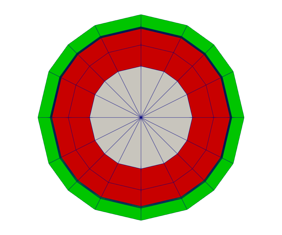
Figure 2: Solid mesh for the OpenMC and heat conduction problems. Red and white: UO2 fuel. Green: Zr clad.
To generate the mesh, run
cardinal-opt -i solid_mesh.i --mesh-only
Neutronics Input File
The neutronics physics is solved over the entire domain using OpenMC; the OpenMC wrapping is described in openmc.i. We begin by loading the mesh that OpenMC will receive temperature from the coupled MOOSE application, and on which OpenMC will write the fission heat source:
[Mesh<<<{"href": "../syntax/Mesh/index.html"}>>>]
  [file]
    type = FileMeshGenerator<<<{"description": "Read a mesh from a file.", "href": "../source/meshgenerators/FileMeshGenerator.html"}>>>
    file<<<{"description": "The filename to read."}>>> = solid_mesh_in.e
  []
[]Next, we define an AuxVariable to visualize the temperature Cardinal is setting in OpenMC cells, and write to it with a CellTemperatureAux (which queries the cell temperature in the OpenMC geometry):
[AuxVariables<<<{"href": "../syntax/AuxVariables/index.html"}>>>]
  [cell_temperature]
    family<<<{"description": "Specifies the family of FE shape functions to use for this variable"}>>> = MONOMIAL
    order<<<{"description": "Specifies the order of the FE shape function to use for this variable (additional orders not listed are allowed)"}>>> = CONSTANT
  []
[]

[AuxKernels<<<{"href": "../syntax/AuxKernels/index.html"}>>>]
  [cell_temperature]
    type = CellTemperatureAux<<<{"description": "OpenMC cell temperature (K), mapped to each MOOSE element", "href": "../source/auxkernels/CellTemperatureAux.html"}>>>
    variable<<<{"description": "The name of the variable that this object applies to"}>>> = cell_temperature
  []
[]Afterwards, we replace the default finite element problem with an OpenMCCellAverageProblem. This class is responsible for initializing OpenMC, setting cell temperatures and densities (with equivalent field variables on the [Mesh]), and writing results from OpenMC tallies to the MOOSE mesh. We start by overriding the number of inactive batches, the total number of batches, and the number of particles per batch. It should be noted that these settings can be applied in make_openmc_model.py when generating the OpenMC model as well. A large number of inactive batches (in this case, 400) are required when running TRRM as both the scattering and fission sources must be converged. Fewer rays per batch (1000 in this case) are required as rays do not terminate until they reach the end of the active length (unlike particles, which are killed on absorption). We then specify scaling = 100.0 to convert from mesh units (m) to OpenMC units (cm). We also set the pin power used to normalize tally scores. Afterwards, we set the depth in the OpenMC geometry we wish to couple to (cell_level), and specify that we wish to couple OpenMC to the fuel (uo2 and uo2_tri blocks) with temperature feedback. To speed up the rate of convergence and avoid the nonlinear feedback instabilities commonly observed in LWR multiphysics calculations, we use constant relaxation with a relaxation factor of 0.5. The final component of the OpenMC problem setup is to add a CellTally which accumulates kappa_fission over uo2 and uo2_tri. In addition to fission heating tally value, we enable outputs for the heating standard deviation and relative error.
[Problem<<<{"href": "../syntax/Problem/index.html"}>>>]
  type = OpenMCCellAverageProblem
  particles = 1000
  inactive_batches = 400
  batches = 800

  scaling = 100.0

  power = ${P_PIN}

  cell_level = 1
  temperature_blocks = 'uo2_tri uo2'

  relaxation = 'constant'
  relaxation_factor = 0.5

  [Tallies<<<{"href": "../syntax/Problem/Tallies/index.html"}>>>]
    [heating]
      type = CellTally<<<{"description": "A class which implements distributed cell tallies.", "href": "../source/tallies/CellTally.html"}>>>
      score<<<{"description": "Score(s) to use in the OpenMC tallies. If not specified, defaults to 'kappa_fission'"}>>> = 'kappa_fission'
      output<<<{"description": "UNRELAXED field(s) to output from OpenMC for each tally score. unrelaxed_tally_std_dev will write the standard deviation of each tally into auxiliary variables named *_std_dev. unrelaxed_tally_rel_error will write the relative standard deviation (unrelaxed_tally_std_dev / unrelaxed_tally) of each tally into auxiliary variables named *_rel_error. unrelaxed_tally will write the raw unrelaxed tally into auxiliary variables named *_raw (replace * with 'name')."}>>> = 'unrelaxed_tally_std_dev unrelaxed_tally_rel_error'
      block<<<{"description": "Subdomains for which to add tallies in OpenMC. If not provided, tallies will be applied over the entire domain corresponding to the [Mesh] block."}>>> = 'uo2 uo2_tri'
    []
  []
[]The specification of temperature blocks in the [Problem] will add a variable named temp to the mesh, which the OpenMCCellAverageProblem will query to set cell temperatures. To avoid an initial temperature of zero being sent to OpenMC, we add a ConstantIC which sets this field variable to the average fluid temperature:
[ICs<<<{"href": "../syntax/Cardinal/ICs/index.html"}>>>]
  [temp_fuel]
    type = ConstantIC<<<{"description": "Sets a constant field value.", "href": "../source/ics/ConstantIC.html"}>>>
    variable<<<{"description": "The variable this initial condition is supposed to provide values for."}>>> = temp
    value<<<{"description": "The value to be set in IC"}>>> = '${T_AVG}'
  []
[]The next set of blocks we add sets up the coupling scheme. We add a TransientMultiApp for the heat conduction solve, which receives fission heating from heat_source_to_solid (a MultiAppGeneralFieldShapeEvaluationTransfer) and sends the fuel temperature to temp via temp_to_openmc (another MultiAppGeneralFieldShapeEvaluationTransfer). The heat conduction application is executed after running OpenMC (on TIMESTEP_END), resulting in the following coupling scheme:
Run OpenMC;
Send fission power to heat conduction application (
solid);Compute fuel temperatures;
Send fuel temperatures back to OpenMC;
Repeat until fields are converged.
[MultiApps<<<{"href": "../syntax/MultiApps/index.html"}>>>]
  [solid]
    type = TransientMultiApp<<<{"description": "MultiApp for performing coupled simulations with the parent and sub-application both progressing in time.", "href": "../source/multiapps/TransientMultiApp.html"}>>>
    input_files<<<{"description": "The input file for each App.  If this parameter only contains one input file it will be used for all of the Apps.  When using 'positions_from_file' it is also admissable to provide one input_file per file."}>>> = 'solid.i'
    execute_on<<<{"description": "The list of flag(s) indicating when this object should be executed. For a description of each flag, see https://mooseframework.inl.gov/source/interfaces/SetupInterface.html."}>>> = timestep_end
  []
[]

[Transfers<<<{"href": "../syntax/Transfers/index.html"}>>>]
  [heat_source_to_solid]
    type = MultiAppGeneralFieldShapeEvaluationTransfer<<<{"description": "Transfers field data at the MultiApp position using the finite element shape functions from the origin application.", "href": "../source/transfers/MultiAppGeneralFieldShapeEvaluationTransfer.html"}>>>
    to_multi_app<<<{"description": "The name of the MultiApp to transfer the data to"}>>> = solid
    variable<<<{"description": "The auxiliary variable to store the transferred values in."}>>> = heat_source
    source_variable<<<{"description": "The variable to transfer from."}>>> = kappa_fission
    from_postprocessors_to_be_preserved<<<{"description": "The name of the Postprocessor in the from-app to evaluate an adjusting factor."}>>> = source_integral
    to_postprocessors_to_be_preserved<<<{"description": "The name of the Postprocessor in the to-app to evaluate an adjusting factor."}>>> = source_integral
    from_blocks<<<{"description": "Subdomain restriction to transfer from (defaults to all the origin app domain)"}>>> = 'uo2_tri uo2'
    to_blocks<<<{"description": "Subdomain restriction to transfer to, (defaults to all the target app domain)"}>>> = 'uo2_tri uo2'
  []
  [temp_to_openmc]
    type = MultiAppGeneralFieldShapeEvaluationTransfer<<<{"description": "Transfers field data at the MultiApp position using the finite element shape functions from the origin application.", "href": "../source/transfers/MultiAppGeneralFieldShapeEvaluationTransfer.html"}>>>
    from_multi_app<<<{"description": "The name of the MultiApp to receive data from"}>>> = solid
    variable<<<{"description": "The auxiliary variable to store the transferred values in."}>>> = temp
    source_variable<<<{"description": "The variable to transfer from."}>>> = temp
    from_blocks<<<{"description": "Subdomain restriction to transfer from (defaults to all the origin app domain)"}>>> = 'uo2_tri uo2'
    to_blocks<<<{"description": "Subdomain restriction to transfer to, (defaults to all the target app domain)"}>>> = 'uo2_tri uo2'
  []
[]The final portion of the input file deals with execution, post-processing, and outputs. We use a Transient executioner in this problem to control the number of iterations between the OpenMC main application and the heat conduction sub-application. In this problem, 5 iterations are sufficient to converge tally statistics and due to the low variance of TRRM. It should be noted that the problem OpenMC is solving is still a quasi-static k-eigenvalue calculation, and the heat conduction simulation is a steady-state governing equation with the use of a Transient executioner. We add a series of post-processors to monitor the relative errors of tally variables and report the k-eigenvalue (and its associated standard deviation). Finally, we select Exodus and CSV output in the [Outputs] block.
[Postprocessors<<<{"href": "../syntax/Postprocessors/index.html"}>>>]
  [max_rel_err]
    type = TallyRelativeError<<<{"description": "Maximum/minimum tally relative error", "href": "../source/postprocessors/TallyRelativeError.html"}>>>
    value_type<<<{"description": "Whether to give the maximum or minimum tally relative error"}>>> = max
    tally_score<<<{"description": "Score to report the relative error. If there is just a single score, this defaults to that value"}>>> = kappa_fission
  []
  [min_rel_err]
    type = TallyRelativeError<<<{"description": "Maximum/minimum tally relative error", "href": "../source/postprocessors/TallyRelativeError.html"}>>>
    value_type<<<{"description": "Whether to give the maximum or minimum tally relative error"}>>> = min
    tally_score<<<{"description": "Score to report the relative error. If there is just a single score, this defaults to that value"}>>> = kappa_fission
  []
  [avg_rel_err]
    type = TallyRelativeError<<<{"description": "Maximum/minimum tally relative error", "href": "../source/postprocessors/TallyRelativeError.html"}>>>
    value_type<<<{"description": "Whether to give the maximum or minimum tally relative error"}>>> = average
    tally_score<<<{"description": "Score to report the relative error. If there is just a single score, this defaults to that value"}>>> = kappa_fission
  []

  [k]
    type = KEigenvalue<<<{"description": "k eigenvalue computed by OpenMC", "href": "../source/postprocessors/KEigenvalue.html"}>>>
    output<<<{"description": "The value to output. Options are $k_{eff}$ (mean), the standard deviation of $k_{eff}$ (std_dev), or the relative error of $k_{eff}$ (rel_err)."}>>> = 'mean'
    value_type<<<{"description": "Type of eigenvalue global tally to report"}>>> = 'tracklength'
  []
  [k_std_dev]
    type = KEigenvalue<<<{"description": "k eigenvalue computed by OpenMC", "href": "../source/postprocessors/KEigenvalue.html"}>>>
    output<<<{"description": "The value to output. Options are $k_{eff}$ (mean), the standard deviation of $k_{eff}$ (std_dev), or the relative error of $k_{eff}$ (rel_err)."}>>> = 'std_dev'
    value_type<<<{"description": "Type of eigenvalue global tally to report"}>>> = 'tracklength'
  []

  [source_integral]
    type = ElementIntegralVariablePostprocessor<<<{"description": "Computes a volume integral of the specified variable", "href": "../source/postprocessors/ElementIntegralVariablePostprocessor.html"}>>>
    variable<<<{"description": "The name of the variable that this object operates on"}>>> = kappa_fission
    execute_on<<<{"description": "The list of flag(s) indicating when this object should be executed. For a description of each flag, see https://mooseframework.inl.gov/source/interfaces/SetupInterface.html."}>>> = 'TRANSFER TIMESTEP_END'
    block<<<{"description": "The list of blocks (ids or names) that this object will be applied"}>>> = 'uo2_tri uo2'
  []
[]

[Executioner<<<{"href": "../syntax/Executioner/index.html"}>>>]
  type = Transient
  num_steps = 5
[]

[Outputs<<<{"href": "../syntax/Outputs/index.html"}>>>]
  execute_on<<<{"description": "The list of flag(s) indicating when this object should be executed. For a description of each flag, see https://mooseframework.inl.gov/source/interfaces/SetupInterface.html."}>>> = 'timestep_end'
  exodus<<<{"description": "Output the results using the default settings for Exodus output."}>>> = true
  csv<<<{"description": "Output the scalar variable and postprocessors to a *.csv file using the default CSV output."}>>> = true
[]Solid Input File
The heat conduction problem is setup in the solid.i input file, and is very similar to the continuous energy LWR pincell tutorial. It begins by loading the previously generated mesh.
[Mesh<<<{"href": "../syntax/Mesh/index.html"}>>>]
  [File]
    type = FileMeshGenerator<<<{"description": "Read a mesh from a file.", "href": "../source/meshgenerators/FileMeshGenerator.html"}>>>
    file<<<{"description": "The filename to read."}>>> = solid_mesh_in.e
  []
[]Afterwards, nonlinear and auxiliary variables are added for the temperature and heat source (respectively). This is followed by the addition of kernels to assemble the heat conduction equation over the fuel and cladding (where the fission heat source heat is block restricted to the fuel).
[Variables<<<{"href": "../syntax/Variables/index.html"}>>>]
  [temp]
    initial_condition<<<{"description": "Specifies a constant initial condition for this variable"}>>> = ${T_AVG}
  []
[]

[AuxVariables<<<{"href": "../syntax/AuxVariables/index.html"}>>>]
  [heat_source]
    family<<<{"description": "Specifies the family of FE shape functions to use for this variable"}>>> = MONOMIAL
    order<<<{"description": "Specifies the order of the FE shape function to use for this variable (additional orders not listed are allowed)"}>>> = CONSTANT
    block = 'uo2_tri uo2'
  []
[]

[Kernels<<<{"href": "../syntax/Kernels/index.html"}>>>]
  [hc]
    type = HeatConduction<<<{"description": "Diffusive heat conduction term $-\\nabla\\cdot(k\\nabla T)$ of the thermal energy conservation equation", "href": "../source/kernels/HeatConduction.html"}>>>
    variable<<<{"description": "The name of the variable that this residual object operates on"}>>> = temp
    block<<<{"description": "The list of blocks (ids or names) that this object will be applied"}>>> = 'uo2_tri uo2 clad'
  []
  [heat]
    type = CoupledForce<<<{"description": "Implements a source term proportional to the value of a coupled variable. Weak form: $(\\psi_i, -\\sigma v)$.", "href": "../source/kernels/CoupledForce.html"}>>>
    variable<<<{"description": "The name of the variable that this residual object operates on"}>>> = temp
    v<<<{"description": "The coupled variable which provides the force"}>>> = heat_source
    block<<<{"description": "The list of blocks (ids or names) that this object will be applied"}>>> = 'uo2_tri uo2'
  []
[]We then add a ParsedFunction to represent Eq. (2), and a ConvectiveFluxFunction to apply the convective boundary condition to the outer radius of the clad.
[Functions<<<{"href": "../syntax/Functions/index.html"}>>>]
  [T_fluid]
    type = ParsedFunction<<<{"description": "Function created by parsing a string", "href": "../source/functions/MooseParsedFunction.html"}>>>
    expression<<<{"description": "The user defined function."}>>> = '${T_INLET} + ${fparse T_OUTLET - T_INLET} * ((z + ${fparse 0.5 * 1e-2 * HEIGHT}) / ${fparse 1e-2 * HEIGHT})'
  []
[]

[BCs<<<{"href": "../syntax/BCs/index.html"}>>>]
  [surface]
    type = ConvectiveFluxFunction<<<{"description": "Determines boundary value by fluid heat transfer coefficient and far-field temperature", "href": "../source/bcs/ConvectiveFluxFunction.html"}>>>
    T_infinity<<<{"description": "Function describing far-field temperature"}>>> = T_fluid

    coefficient<<<{"description": "Function describing heat transfer coefficient"}>>> = ${CONV_HT_COEFF}
    variable<<<{"description": "The name of the variable that this residual object operates on"}>>> = temp
    boundary<<<{"description": "The list of boundary IDs from the mesh where this object applies"}>>> = 'clad_or'
  []
[]A series of GenericConstantMaterial are then added to set the thermal conductivity of the fuel and cladding, which is followed by the addition of a GapHeatTransfer to set up the gap conductance model.
[Materials<<<{"href": "../syntax/Materials/index.html"}>>>]
  [k_fuel]
    type = GenericConstantMaterial<<<{"description": "Declares material properties based on names and values prescribed by input parameters.", "href": "../source/materials/GenericConstantMaterial.html"}>>>
    prop_values<<<{"description": "The values associated with the named properties"}>>> = '${K_FUEL}'
    prop_names<<<{"description": "The names of the properties this material will have"}>>> = 'thermal_conductivity'
    block<<<{"description": "The list of blocks (ids or names) that this object will be applied"}>>> = 'uo2_tri uo2'
  []
  [k_clad]
    type = GenericConstantMaterial<<<{"description": "Declares material properties based on names and values prescribed by input parameters.", "href": "../source/materials/GenericConstantMaterial.html"}>>>
    prop_values<<<{"description": "The values associated with the named properties"}>>> = '${K_CLAD}'
    prop_names<<<{"description": "The names of the properties this material will have"}>>> = 'thermal_conductivity'
    block<<<{"description": "The list of blocks (ids or names) that this object will be applied"}>>> = 'clad'
  []
[]

[ThermalContact<<<{"href": "../syntax/ThermalContact/index.html"}>>>]
  # This adds boundary conditions between the fuel and the cladding, which represents
  # the heat flux in both directions as
  # q''= h * (T_1 - T_2)
  # where h is a conductance that accounts for conduction through a material and
  # radiation between two infinite parallel plate gray bodies.
  [one_to_two]
    type = GapHeatTransfer
    variable = temp
    primary = 'fuel_or'
    secondary = 'clad_ir'

    # we will use a quadrature-based approach to find the gap width and cross-side temperature
    quadrature = true

    # emissivity of the fuel
    emissivity_primary = 0.8

    # emissivity of the clad
    emissivity_secondary = 0.8

    # thermal conductivity of the gap material
    gap_conductivity = ${K_GAS}

    # geometric terms related to the gap
    gap_geometry_type = CYLINDER
    cylinder_axis_point_1 = '0 0 ${fparse -0.5 * 1e-2 * HEIGHT}'
    cylinder_axis_point_2 = '0 0 ${fparse  0.5 * 1e-2 * HEIGHT}'
  []
[]Finally, the [Executioner] is set to Transient. As no timestepping parameters are provided, the heat conduction simulation will execute in lock-step with the OpenMC simulation because sub_cycling = true was set in the openmc.i file. We add several post-processors to monitor the maximum fuel and cladding temperatures, and select Exodus and CSV output in the [Outputs] block.
[Executioner<<<{"href": "../syntax/Executioner/index.html"}>>>]
  type = Transient
  nl_abs_tol = 1e-8
  petsc_options_iname = '-pc_type -pc_hypre_type'
  petsc_options_value = 'hypre boomeramg'
[]

[Postprocessors<<<{"href": "../syntax/Postprocessors/index.html"}>>>]
  [source_integral]
    type = ElementIntegralVariablePostprocessor<<<{"description": "Computes a volume integral of the specified variable", "href": "../source/postprocessors/ElementIntegralVariablePostprocessor.html"}>>>
    variable<<<{"description": "The name of the variable that this object operates on"}>>> = heat_source
    execute_on<<<{"description": "The list of flag(s) indicating when this object should be executed. For a description of each flag, see https://mooseframework.inl.gov/source/interfaces/SetupInterface.html."}>>> = 'TRANSFER TIMESTEP_END'
    block<<<{"description": "The list of blocks (ids or names) that this object will be applied"}>>> = 'uo2_tri uo2'
  []
  [max_fuel_T]
    type = NodalExtremeValue<<<{"description": "Finds either the min or max elemental value of a variable over the domain.", "href": "../source/postprocessors/NodalExtremeValue.html"}>>>
    variable<<<{"description": "The name of the variable that this postprocessor operates on"}>>> = temp
    block<<<{"description": "The list of blocks (ids or names) that this object will be applied"}>>> = 'uo2_tri uo2'
  []
  [max_clad_T]
    type = NodalExtremeValue<<<{"description": "Finds either the min or max elemental value of a variable over the domain.", "href": "../source/postprocessors/NodalExtremeValue.html"}>>>
    variable<<<{"description": "The name of the variable that this postprocessor operates on"}>>> = temp
    block<<<{"description": "The list of blocks (ids or names) that this object will be applied"}>>> = 'clad'
  []
[]

[Outputs<<<{"href": "../syntax/Outputs/index.html"}>>>]
  exodus<<<{"description": "Output the results using the default settings for Exodus output."}>>> = true
  execute_on<<<{"description": "The list of flag(s) indicating when this object should be executed. For a description of each flag, see https://mooseframework.inl.gov/source/interfaces/SetupInterface.html."}>>> = 'TIMESTEP_END'
  csv<<<{"description": "Output the scalar variable and postprocessors to a *.csv file using the default CSV output."}>>> = true
[]Execution and Postprocessing
To run the coupled calculation with TRRM and flat sources,
python make_openmc_model.py -r
cardinal-opt -i solid_mesh.i --mesh-only
cardinal-opt -i openmc.i --n-threads=4
To run with TRRM and linear sources,
python make_openmc_model.py -r --linear
cardinal-opt -i solid_mesh.i --mesh-only
cardinal-opt -i openmc.i --n-threads=4
and to run the continuous energy reference,
python make_openmc_model.py
cardinal-opt -i solid_mesh.i --mesh-only
cardinal-opt -i openmc.i --n-threads=4
All of the above will use 4 OpenMP threads. To run the simulation faster, you can increase the number of OpenMP threads or decrease the number of particles. Bear in mind that decreasing the number of particles may result in a failure to converge when running TRRM as fewer source regions will be hit on each power iteration. The TRRM solver does not support distributed memory calculations yet, and so adding extra MPI ranks will not speed up the neutronics calculation as all work is done by rank zero.
Table 2 shows the resulting k-eigenvalues for each TRRM discretization approach compared against the continuous energy reference (10000 particles per batch, 1100 batches, 100 inactive batches) on the first Picard iteration before multiphysics feedback is applied. In general, the single physics TRRM calculations agree quite well with the continuous energy reference (within three standard deviations). Table 3 shows the k-eigenvalues for each case on the final Picard iteration; the agreement is less than stellar and can be attributed to the use of isothermal temperature interpolation tables in the multiphysics model.
Table 2: k-eigenvalue predictions on the initial Picard iteration.
| Method | (PCM) | |
|---|---|---|
| CE Monte Carlo | N/A | |
| Flat Source | ||
| Linear Source |
Table 3: k-eigenvalue predictions on the final Picard iteration.
| Method | (PCM) | |
|---|---|---|
| CE Monte Carlo | N/A | |
| Flat Source | ||
| Linear Source |
Figure 3 plots the center-plane radial fission heating distribution for the different spatial discretization schemes and compares them with the continuous energy reference on the final Picard iteration. There is a fairly large discrepancy (up to 10%) which is caused by over-exaggerated Doppler broadening in the fuel, depressing the center plane power compared to the continuous energy result. We can confirm this trend by plotting the axial centerline power distribution in Figure 4. This shows a 10% under-prediction of power in the core center followed by an over-prediction as one moves from the core center towards the vacuum boundary condition. This showcases the need for reasonable MGXS temperature interpolation tables in multiphysics calculations; simple temperature isotherms will not suffice when there are large thermal gradients. Figure 4 also demonstrates the advantage of TRRM - uniform statistical relative errors across the problem domain. This is advantageous for whole-core calculations where Monte Carlo transport struggles to steer particles to the core periphery.
 spatial discretization approaches against continuous energy Monte Carlo radially.](../media/rr_lwr_radial_comp.png)
Figure 3: Comparison of the different TRRM spatial discretization approaches against continuous energy Monte Carlo radially.
 spatial discretization approaches against continuous energy Monte Carlo axially. Left: fission heating. Right: fission heating statistical relative error.](../media/rr_lwr_axial_comparison.png)
Figure 4: Comparison of the different TRRM spatial discretization approaches against continuous energy Monte Carlo axially. Left: fission heating. Right: fission heating statistical relative error.
References
- S. Cathalau, J. C. Lefebvre, and J. P. West.
Proposal for a Second Stage of the Benchmark on Power Distributions within Assemblies.
Technical Report NEA/NSC/DOC(96)2, Organisation for Economic Cooperation and Development, Nuclear Energy Agency, 1996.
URL: https://www.oecd-nea.org/upload/docs/application/pdf/2020-01/nsc-doc96-02-rev2.pdf.[Export]
- M.A. Smith, E.E. Lewis, and Byung-Chan Na.
Benchmark on Deterministic 3-D MOX Fuel Assembly Transport Calculations without Spatial Homogenization.
Progress in Nuclear Energy, 48(5):383–393, 2006.
doi:https://doi.org/10.1016/j.pnucene.2006.01.002.[Export]