DAGMC pincell
In this tutorial, you will learn how to:
Couple CAD Monte Carlo models via temperature and heat source feedback to MOOSE
To access this tutorial,
cd cardinal/tutorials/dagmc
To run this tutorial, you need to have built Cardinal with DAGMC support enabled, by setting export ENABLE_DAGMC=true.
Geometry and Computational Models
This model consists of a pincell, taken directly from an OpenMC DAGMC tutorial. DAGMC is a package for Monte Carlo transport on Computer Aided Design (CAD) geometry. We will not go into detail on how the DAGMC model was generated, but instead refer you to the DAGMC documentation.
The geometry consists of a U-235 cylinder enclosed in an annulus of water. The height is 40 cm, and the outer diameter of the fuel cylinder is 18 cm. The total power is set to 1000 W. An image of the geometry is shown on the - plane in Figure 1.

Figure 1: OpenMC DAGMC geometry colored by material, on the - plane.
Figure 2 shows the same DAGMC model, colored instead by cell. The two green regions are both U-235, while the purple is water. There is no particular reason why the model is built this way, since we are just fetching it from an existing OpenMC tutorial.

Figure 2: OpenMC DAGMC geometry colored by cell, on the - plane.
MOOSE Heat Conduction Model
The MOOSE heat transfer module is used to solve for steady-state heat conduction,
(1)
where is the solid thermal conductivity, is the solid temperature, and is a volumetric heat source in the solid.
MeshGenerators are used to construct the solid mesh. Figure 3 shows the solid mesh with block IDs and sidesets. We will not model any heat transfer in the water region, for simplicity. Different block IDs are used for the hexahedral and prism elements in the pellet region because libMesh does not allow different element types to exist on the same block ID. To generate the mesh,
cardinal-opt -i mesh.i --mesh-only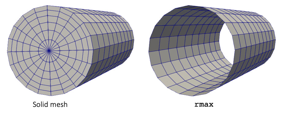
Figure 3: Mesh for the solid portions of a pincell
The surface of the pincell is simply set to a constant value, . Because heat transfer and fluid flow in the borated water is not modeled in this example, The top and bottom of the solid pincell are assumed insulated. In this example, the MOOSE heat transfer module will run first. The initial solid temperature is 500°C and the initial power is zero.
OpenMC Model
The OpenMC model is built using DAGMC. Particles move through space with surface-to-surface tracking between triangle surface meshes. Cells are the regions of space enclosed by these surfaces. After building the DAGMC model with Cubit, we set up the OpenMC input files using the Python API. First, we define materials, then fetch the geometry from the DAGMC geometry file (dagmc.h5m). Then, we set up the settings, for numbers of batches and particles, and how we would like to have temperature feedback applied to OpenMC.
import openmc

# materials
u235 = openmc.Material(name="fuel")
u235.add_nuclide('U235', 1.0, 'ao')
u235.set_density('g/cc', 11)
u235.id = 40

water = openmc.Material(name="water")
water.add_nuclide('H1', 2.0, 'ao')
water.add_nuclide('O16', 1.0, 'ao')
water.set_density('g/cc', 1.0)
water.add_s_alpha_beta('c_H_in_H2O')
water.id = 41

mats = openmc.Materials([u235, water])
mats.export_to_xml()

dagmc_univ = openmc.DAGMCUniverse(filename="dagmc.h5m")
geometry = openmc.Geometry(root=dagmc_univ)
geometry.export_to_xml()

settings = openmc.Settings()
settings.dagmc = True
settings.batches = 10
settings.inactive = 2
settings.particles = 5000

settings.temperature = {'default': 500.0,
                        'method': 'interpolation',
                        'range': (294.0, 3000.0),
                        'tolerance': 1000.0}

settings.export_to_xml()

settings.source = openmc.IndependentSource(space=openmc.stats.Box([-4., -4., -4.],
                                                       [ 4.,  4.,  4.]))
settings.export_to_xml()

p1 = openmc.Plot()
p1.filename = 'plot1'
p1.basis = 'xy'
p1.width = (25.0, 25.0)
p1.pixels = (400, 400)
p1.color_by = 'material'
p1.colors = {u235: 'yellow', water: 'blue'}

p2 = openmc.Plot()
p2.filename = 'plot2'
p2.basis = 'xy'
p2.width = (18.0, 18.0)
p2.pixels = (400, 400)
p2.color_by = 'cell'

plots = openmc.Plots([p1, p2])
plots.export_to_xml()
To generate the XML files needed to run OpenMC, you can run the following:
python make_model.py
or simply use the XML files checked in to the tutorials/dagmc directory.
Multiphysics Coupling
In this section, OpenMC and MOOSE are coupled for heat source and temperature feedback for a DAGMC pincell. The following sub-sections describe these files.
Solid Input Files
The solid phase is solved with the MOOSE heat transfer module, and is described in the solid.i input. The solid mesh is created using mesh generators in the mesh.i input:
r_pin = ${fparse 18 / 2.0}
L = 40.0

[Mesh<<<{"href": "../syntax/Mesh/index.html"}>>>]
  [fuel] # this makes a circle that will represent the fuel
    type = AnnularMeshGenerator<<<{"description": "For rmin>0: creates an annular mesh of QUAD4 elements. For rmin=0: creates a disc mesh of QUAD4 and TRI3 elements. Boundary sidesets are created at rmax and rmin, and given these names. If dmin!=0 and dmax!=360, a sector of an annulus or disc is created. In this case boundary sidesets are also created at dmin and dmax, and given these names", "href": "../source/meshgenerators/AnnularMeshGenerator.html"}>>>
    nr<<<{"description": "Number of elements in the radial direction"}>>> = 9
    nt<<<{"description": "Number of elements in the angular direction"}>>> = 20
    rmin<<<{"description": "Inner radius.  If rmin=0 then a disc mesh (with no central hole) will be created."}>>> = 0
    rmax<<<{"description": "Outer radius"}>>> = ${r_pin}
    quad_subdomain_id<<<{"description": "The subdomain ID given to the QUAD4 elements"}>>> = 2
    tri_subdomain_id<<<{"description": "The subdomain ID given to the TRI3 elements (these exist only if rmin=0, and they exist at the center of the disc"}>>> = 3
  []
  [extrude] # this extrudes the circle in the axial direction
    type = AdvancedExtruderGenerator<<<{"description": "Extrudes a 1D mesh into 2D, or a 2D mesh into 3D, and supports a variable height for each elevation, variable number of layers within each elevation, variable growth factors of axial element sizes within each elevation and remap subdomain_ids, boundary_ids and element extra integers within each elevation as well as interface boundaries between neighboring elevation layers, as well as following a 1D curve and modifying the radial (normal to the extrusion axis) extent of the geometry.", "href": "../source/meshgenerators/AdvancedExtruderGenerator.html"}>>>
    input<<<{"description": "The mesh to extrude"}>>> = fuel
    heights<<<{"description": "The height of each elevation"}>>> = '${L}'
    num_layers<<<{"description": "The number of layers for each elevation - must be num_elevations in length!"}>>> = '10'
    direction<<<{"description": "A vector that points in the direction to extrude (note, this will be normalized internally - so don't worry about it here)"}>>> = '0 0 1'
  []
  [shift]
    type = TransformGenerator<<<{"description": "Applies a linear transform to the entire mesh.", "href": "../source/meshgenerators/TransformGenerator.html"}>>>
    input<<<{"description": "The mesh we want to modify"}>>> = extrude
    transform<<<{"description": "The type of transformation to perform (TRANSLATE, TRANSLATE_CENTER_ORIGIN, TRANSLATE_MIN_ORIGIN, ROTATE, SCALE, ROTATE_WITH_MATRIX, ROTATE_EXT)"}>>> = translate
    vector_value<<<{"description": "The value to use for the transformation. When using TRANSLATE or SCALE, the xyz coordinates are applied in each direction respectively. When using ROTATE, the values are interpreted as the Euler angles phi, theta and psi given in degrees. For ROTATE_EXT, an extrinsic rotation is carried out using prescribed Euler angles alpha, beta, and gamma in degrees."}>>> = '0.0 0.0 ${fparse -1.0 * L / 2.0}'
  []
[]We generate the mesh by running cardinal-opt -i mesh.i --mesh-only to create the mesh_in.e file, which we then use in the solid input file.
[Mesh<<<{"href": "../syntax/Mesh/index.html"}>>>]
  [file]
    type = FileMeshGenerator<<<{"description": "Read a mesh from a file.", "href": "../source/meshgenerators/FileMeshGenerator.html"}>>>
    file<<<{"description": "The filename to read."}>>> = mesh_in.e
  []
[]The heat transfer module will solve for temperature, with the heat equation. The variables, kernels, and boundary conditions are shown below.
[Variables<<<{"href": "../syntax/Variables/index.html"}>>>]
  [temp]
    initial_condition<<<{"description": "Specifies a constant initial condition for this variable"}>>> = 500.0
  []
[]

[AuxVariables<<<{"href": "../syntax/AuxVariables/index.html"}>>>]
  [heat_source]
    family<<<{"description": "Specifies the family of FE shape functions to use for this variable"}>>> = MONOMIAL
    order<<<{"description": "Specifies the order of the FE shape function to use for this variable (additional orders not listed are allowed)"}>>> = CONSTANT
  []
[]

[Kernels<<<{"href": "../syntax/Kernels/index.html"}>>>]
  [hc]
    type = HeatConduction<<<{"description": "Diffusive heat conduction term $-\\nabla\\cdot(k\\nabla T)$ of the thermal energy conservation equation", "href": "../source/kernels/HeatConduction.html"}>>>
    variable<<<{"description": "The name of the variable that this residual object operates on"}>>> = temp
  []
  [heat]
    type = CoupledForce<<<{"description": "Implements a source term proportional to the value of a coupled variable. Weak form: $(\\psi_i, -\\sigma v)$.", "href": "../source/kernels/CoupledForce.html"}>>>
    variable<<<{"description": "The name of the variable that this residual object operates on"}>>> = temp
    v<<<{"description": "The coupled variable which provides the force"}>>> = heat_source
  []
[]

[BCs<<<{"href": "../syntax/BCs/index.html"}>>>]
  [surface]
    type = DirichletBC<<<{"description": "Imposes the essential boundary condition $u=g$, where $g$ is a constant, controllable value.", "href": "../source/bcs/DirichletBC.html"}>>>
    variable<<<{"description": "The name of the variable that this residual object operates on"}>>> = temp
    boundary<<<{"description": "The list of boundary IDs from the mesh where this object applies"}>>> = 'rmax'
    value<<<{"description": "Value of the BC"}>>> = 500.0
  []
[]

[Materials<<<{"href": "../syntax/Materials/index.html"}>>>]
  [k_fuel]
    type = GenericConstantMaterial<<<{"description": "Declares material properties based on names and values prescribed by input parameters.", "href": "../source/materials/GenericConstantMaterial.html"}>>>
    prop_values<<<{"description": "The values associated with the named properties"}>>> = '0.05'
    prop_names<<<{"description": "The names of the properties this material will have"}>>> = 'thermal_conductivity'
    block<<<{"description": "The list of blocks (ids or names) that this object will be applied"}>>> = '2 3'
  []
[]The Transfer system in MOOSE is used to communicate variables across applications; a heat source will be computed by OpenMC and applied as a source term in MOOSE. In the opposite direction, MOOSE will compute a temperature that will be applied to the OpenMC geometry. The heat_source auxiliary variable will simply receive the heat source from OpenMC. The MultiApps and Transfers blocks describe the interaction between Cardinal and MOOSE. The MOOSE heat conduction application is run as the main application, with OpenMC run as the sub-application. We specify that MOOSE will run first on each time step.
Two transfers are required to couple OpenMC and MOOSE for heat source and temperature feedback. The first is a transfer of heat source from Cardinal to MOOSE. The second is transfer of temperature from MOOSE to Cardinal.
[MultiApps<<<{"href": "../syntax/MultiApps/index.html"}>>>]
  [openmc]
    type = TransientMultiApp<<<{"description": "MultiApp for performing coupled simulations with the parent and sub-application both progressing in time.", "href": "../source/multiapps/TransientMultiApp.html"}>>>
    input_files<<<{"description": "The input file for each App.  If this parameter only contains one input file it will be used for all of the Apps.  When using 'positions_from_file' it is also admissable to provide one input_file per file."}>>> = 'openmc.i'
    execute_on<<<{"description": "The list of flag(s) indicating when this object should be executed. For a description of each flag, see https://mooseframework.inl.gov/source/interfaces/SetupInterface.html."}>>> = timestep_end
  []
[]

[Transfers<<<{"href": "../syntax/Transfers/index.html"}>>>]
  [heat_source_from_openmc]
    type = MultiAppGeneralFieldShapeEvaluationTransfer<<<{"description": "Transfers field data at the MultiApp position using the finite element shape functions from the origin application.", "href": "../source/transfers/MultiAppGeneralFieldShapeEvaluationTransfer.html"}>>>
    from_multi_app<<<{"description": "The name of the MultiApp to receive data from"}>>> = openmc
    variable<<<{"description": "The auxiliary variable to store the transferred values in."}>>> = heat_source
    source_variable<<<{"description": "The variable to transfer from."}>>> = heat_source
    from_postprocessors_to_be_preserved<<<{"description": "The name of the Postprocessor in the from-app to evaluate an adjusting factor."}>>> = heat_source
    to_postprocessors_to_be_preserved<<<{"description": "The name of the Postprocessor in the to-app to evaluate an adjusting factor."}>>> = source_integral
  []
  [temp_to_openmc]
    type = MultiAppGeneralFieldShapeEvaluationTransfer<<<{"description": "Transfers field data at the MultiApp position using the finite element shape functions from the origin application.", "href": "../source/transfers/MultiAppGeneralFieldShapeEvaluationTransfer.html"}>>>
    to_multi_app<<<{"description": "The name of the MultiApp to transfer the data to"}>>> = openmc
    variable<<<{"description": "The auxiliary variable to store the transferred values in."}>>> = temp
    source_variable<<<{"description": "The variable to transfer from."}>>> = temp
  []
[]For the heat source transfer from OpenMC, we ensure conservation by requiring that the integral of heat source computed by OpenMC (in the heat_source postprocessor) matches the integral of the heat source received by MOOSE (in the source_integral postprocessor). We also add a postprocessor to evaluate the maximum solid temperature.
[Postprocessors<<<{"href": "../syntax/Postprocessors/index.html"}>>>]
  [source_integral]
    type = ElementIntegralVariablePostprocessor<<<{"description": "Computes a volume integral of the specified variable", "href": "../source/postprocessors/ElementIntegralVariablePostprocessor.html"}>>>
    variable<<<{"description": "The name of the variable that this object operates on"}>>> = heat_source
    execute_on<<<{"description": "The list of flag(s) indicating when this object should be executed. For a description of each flag, see https://mooseframework.inl.gov/source/interfaces/SetupInterface.html."}>>> = transfer
  []
  [max_T]
    type = NodalExtremeValue<<<{"description": "Finds either the min or max elemental value of a variable over the domain.", "href": "../source/postprocessors/NodalExtremeValue.html"}>>>
    variable<<<{"description": "The name of the variable that this postprocessor operates on"}>>> = temp
  []
[]Because we did not specify sub-cycling in the [MultiApps] block, this means that OpenMC will run for exactly the same number of time steps (but the actual time step size used by the OpenMC wrapping is of no consequence because OpenMC is run in -eigenvalue mode). By setting a fixed number of time steps, this example will simply run a fixed number of Picard iterations.
[Executioner<<<{"href": "../syntax/Executioner/index.html"}>>>]
  type = Transient
  nl_abs_tol = 1e-8
  num_steps = 3
  petsc_options_iname = '-pc_type -pc_hypre_type'
  petsc_options_value = 'hypre boomeramg'
[]

[Outputs<<<{"href": "../syntax/Outputs/index.html"}>>>]
  exodus<<<{"description": "Output the results using the default settings for Exodus output."}>>> = true
  print_linear_residuals<<<{"description": "Enable printing of linear residuals to the screen (Console)"}>>> = false
[]Neutronics Input Files
The neutronics physics is solved over the entire domain using OpenMC. The OpenMC wrapping is described in the openmc.i input file. We begin by defining a mesh on which OpenMC will receive temperature from the coupled MOOSE application, and on which OpenMC will write the fission heat source. In this example, we use exactly the same solid mesh as the coupled MOOSE application; this is not a requirement, and is relaxed in other tutorials.
[Mesh<<<{"href": "../syntax/Mesh/index.html"}>>>]
  [file]
    type = FileMeshGenerator<<<{"description": "Read a mesh from a file.", "href": "../source/meshgenerators/FileMeshGenerator.html"}>>>
    file<<<{"description": "The filename to read."}>>> = mesh_in.e
  []

  allow_renumbering = false
[]Next, the Problem and Tallies blocks describe all objects necessary for the actual neutronics solve. To replace MOOSE finite element calculations with OpenMC particle transport calculations, the OpenMCCellAverageProblem class is used.
[Problem<<<{"href": "../syntax/Problem/index.html"}>>>]
  type = OpenMCCellAverageProblem
  verbose = true
  cell_level = 0
  temperature_blocks = '2 3'

  power = 1000.0
  volume_calculation = vol

  [Tallies<<<{"href": "../syntax/Problem/Tallies/index.html"}>>>]
    [heat_source]
      type = MeshTally<<<{"description": "A class which implements unstructured mesh tallies.", "href": "../source/tallies/MeshTally.html"}>>>
      mesh_template<<<{"description": "Mesh tally template for OpenMC when using mesh tallies; at present, this mesh must exactly match the mesh used in the [Mesh] block because a one-to-one copy is used to get OpenMC's tally results on the [Mesh]."}>>> = mesh_in.e
      name<<<{"description": "Auxiliary variable name(s) to use for OpenMC tallies. If not specified, defaults to the names of the scores"}>>> = heat_source

      check_tally_sum<<<{"description": "Whether to check consistency between the local tallies with a global tally sum. This will require that the integral of the local tally matches a tally with no filters (defined over the entire phase space)."}>>> = false
      normalize_by_global_tally<<<{"description": "Whether to normalize local tallies by a global tally (true) or else by the sum of the local tally (false)"}>>> = false
    []
  []
[]For this example, we specify the total fission power by which to normalize OpenMC's tally results (because OpenMC's tally results are in units of eV/source particle). Next, we indicate which blocks in the [Mesh] should be considered for temperature feedback using temperature_blocks. Here, we specify temperature feedback for the pellet (blocks 2 and 3). During the initialization, OpenMCCellAverageProblem will automatically map from MOOSE elements to OpenMC cells, and store which MOOSE elements are providing temperature feedback. Then when temperature is sent into OpenMC, that mapping is used to compute a volume-average temperature to apply to each OpenMC cell.
This example uses mesh tallies, as indicated by the MeshTally in the [Tallies] block. OpenMCCellAverageProblem will then automatically add the OpenMC mesh tally using the information provided. Finally, we specify the level in the geometry on which the cells exist. Because we don't have any lattices or filled universes in our OpenMC model, the cell level is zero.
At this point, it is important to remind ourselves of the problem setup. OpenMC is tracking particles with surface-to-surface tracking for a tetrahedral mesh (the dagmc.h5m geometry). However, the [Mesh] block is just overlaid on the problem, and we tally on this separate mesh. The two meshes (the tally mesh in the [Mesh] block vs. the DAGMC mesh) are completely unrelated to one another.
Next, we add a series of auxiliary variables for solution visualization (these are not requried for coupling). To help with understanding how the OpenMC model maps to the mesh in the [Mesh] block, we add auxiliary variables to visualize OpenMC's cell temperature (CellTemperatureAux). Cardinal will also automatically output a variable named cell_id (CellIDAux) and a variable named cell_instance ( CellInstanceAux) to show the spatial mapping.
[AuxVariables<<<{"href": "../syntax/AuxVariables/index.html"}>>>]
  [cell_temperature]
    family<<<{"description": "Specifies the family of FE shape functions to use for this variable"}>>> = MONOMIAL
    order<<<{"description": "Specifies the order of the FE shape function to use for this variable (additional orders not listed are allowed)"}>>> = CONSTANT
  []
[]

[AuxKernels<<<{"href": "../syntax/AuxKernels/index.html"}>>>]
  [cell_temperature]
    type = CellTemperatureAux<<<{"description": "OpenMC cell temperature (K), mapped to each MOOSE element", "href": "../source/auxkernels/CellTemperatureAux.html"}>>>
    variable<<<{"description": "The name of the variable that this object applies to"}>>> = cell_temperature
  []
[]Next, we specify an executioner and output settings. Even though OpenMC technically performs a criticality calculation (with no time dependence), we use the transient executioner so that if we wanted to run OpenMC more times than the coupled main application via subcycling, we would have a way to control that.
[Executioner<<<{"href": "../syntax/Executioner/index.html"}>>>]
  type = Transient
[]

[Outputs<<<{"href": "../syntax/Outputs/index.html"}>>>]
  exodus<<<{"description": "Output the results using the default settings for Exodus output."}>>> = true
  csv<<<{"description": "Output the scalar variable and postprocessors to a *.csv file using the default CSV output."}>>> = true
[]Finally, we add a postprocessor to evaluate the total heat source computed by OpenMC and query other parts of the solution.
[Postprocessors<<<{"href": "../syntax/Postprocessors/index.html"}>>>]
  [heat_source]
    type = ElementIntegralVariablePostprocessor<<<{"description": "Computes a volume integral of the specified variable", "href": "../source/postprocessors/ElementIntegralVariablePostprocessor.html"}>>>
    variable<<<{"description": "The name of the variable that this object operates on"}>>> = heat_source
  []
  [k]
    type = KEigenvalue<<<{"description": "k eigenvalue computed by OpenMC", "href": "../source/postprocessors/KEigenvalue.html"}>>>
  []
[]Execution and Postprocessing
To run the coupled calculation,
mpiexec -np 2 cardinal-opt -i solid.i --n-threads=2
This will run both MOOSE and OpenMC with 2 MPI processes and 2 OpenMP threads per rank. To run the simulation faster, you can increase the parallel processes/threads, or simply decrease the number of particles used in OpenMC. When the simulation has completed, you will have created a number of different output files:
solid_out.e, an Exodus output with the solid mesh and solutionsolid_out_openmc0.e, an Exodus output with the OpenMC solution and the data that was ultimately transferred in/out of OpenMC
Figure 4 shows the heat source computed by OpenMC (units of W/cm) and mapped to the MOOSE mesh, the solid temperature computed by MOOSE, and the temperature imposed in OpenMC. The two images showing temperature share a color scale, and are depicted as a slice through the pellet. Because the DAGMC model only has two cells to represent the fuel region, the temperature imposed in OpenMC is a volume average over the elements corresponding to each of those two cells. If you want to resolve the solid temperature with more detail in the OpenMC model, simply add OpenMC cells where finer feedback is desired - or, you can adaptively re-generate the OpenMC cells using the MoabSkinner.
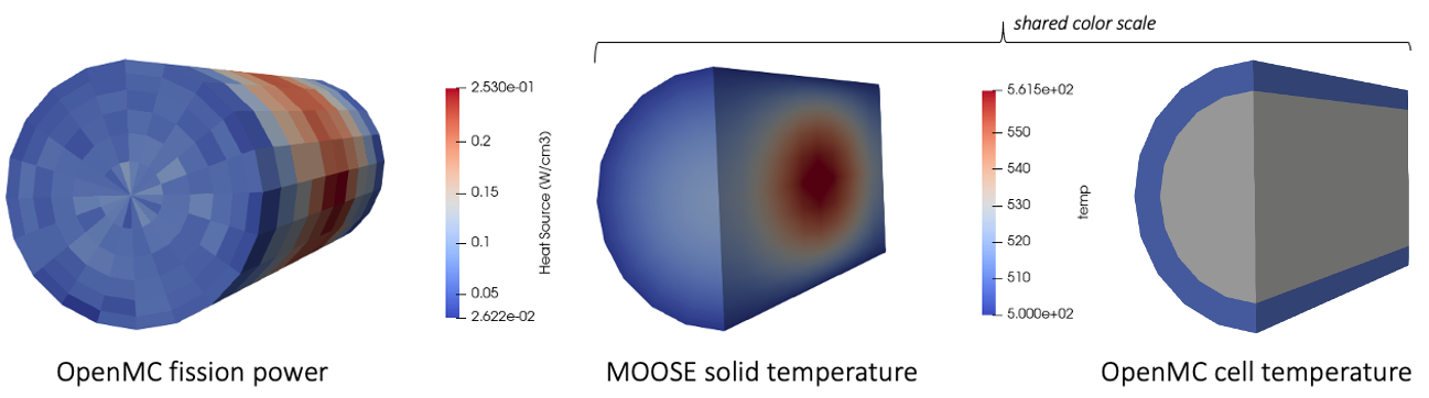
Figure 4: Heat source (W/cm) computed by OpenMC (left); MOOSE solid temperature (middle); OpenMC cell temperature (right)