Multi-Group Cross Section Generation

In this tutorial, you will learn how to generate Multi-Group Cross Sections (MGXS) with distributed cell tallies to couple Cardinal with deterministic transport codes. To access this tutorial,


cd cardinal/tutorials/lwr_mgxs

note:Previous Experience

In this tutorial, we assume the user is familiar with mesh generation via the Reactor module and running Light Water Reactor (LWR) calculations with Cardinal-OpenMC. The LWR AMR tutorial is used as a base for this tutorial; we recommend the LWR AMR tutorial for users not familiar with these concepts.

Geometry and Computational Models

This model consists of a single UO $var element = document.getElementById("moose-equation-94477d45-060d-41d0-a6ec-cea32d4bfa8a");katex.render("_2", element, {displayMode:false,throwOnError:false});$ assembly from the 3D C5G7 extension case in Smith et al. (2006), where control rods are fully inserted in the assembly to induce strong axial and radial gradients. Instead of using the multi-group cross sections from the C5G7 benchmark specifications, the material properties in Cathalau et al. (1996) are used. At a high level the geometry consists of the following lattice elements in a 17x17 grid:

264 fuel pins composed of UO $var element = document.getElementById("moose-equation-0d3f29f7-ef1d-4cee-879c-508c3eddc461");katex.render("_2", element, {displayMode:false,throwOnError:false});$ pellets clad in zirconium with a helium gap;
24 control rods composed of B $var element = document.getElementById("moose-equation-c0d63956-7645-4da0-95d4-cd4b9b32a997");katex.render("_4", element, {displayMode:false,throwOnError:false});$ C pellets clad in aluminum, with no gap, occupying the assembly guide tubes;
A single fission chamber in the central guide tube composed of borated water, with a trace amount of U-235, clad in aluminum with no gap.

The remainder of the assembly not filled with these pincells is composed of borated water. Above the top of the fuel, there is a reflector region which is penetrated by the inserted control rods. The relevant dimensions can be found in Table 1.

Table 1: Geometric specifications for a rodded LWR assembly

Parameter	Value (cm)
Fuel pellet outer radius	0.4095
Fuel clad inner radius	0.418
Fuel clad outer radius	0.475
Control rod outer radius	0.3400
Fission chamber outer radius	0.3400
Guide tube clad outer radius	0.54
Pin pitch	1.26
Fuel height	192.78
Reflector thickness	21.42

When generating MGXS, tallies do not need to be normalized to power, but Cardinal still requires a value of reactor power when performing k-eigenvalue calculations. For this tutorial we select an arbitrary power of 1 W $var element = document.getElementById("moose-equation-cc325536-7177-4810-a946-6a69705b5237");katex.render("_\\text{th}", element, {displayMode:false,throwOnError:false});$ . If you want to compute cross sections accounting for multi-physics feedback, a true reactor power and a coupled thermal-hydraulics solver are required.

OpenMC Model

The OpenMC model follows standard model building practices for LWR geometries. The Python script used to generate the model.xml file can be found below, and a plot of the geometry can be found in Figure 1.


#--------------------------------------------------------------------------------------------------------------------------#
# This is based on the C5G7 reactor physics benchmark problem extension case as described in:                              #
# "Benchmark on Deterministic Transport Calculations Without Spatial Homogenisation: MOX Fuel Assembly 3-D Extension Case" #
# [NEA/NSC/DOC(2005)16]                                                                                                    #
# https://www.oecd-nea.org/upload/docs/application/pdf/2019-12/nsc-doc2005-16.pdf                                          #                                                                                                                     #
#                                                                                                                          #
# The original C5G7 benchmark is defined with multi-group cross sections. To account for                                   #
# continuous energy spectral effects, we chose to use the material properties provided in:                                 #
# "Proposal for a Second Stage of the Benchmark on Power Distributions Within Assemblies"                                  #
# [NEA/NSC/DOC(96)2]                                                                                                       #
# https://www.oecd-nea.org/upload/docs/application/pdf/2020-01/nsc-doc96-02-rev2.pdf                                       #
#--------------------------------------------------------------------------------------------------------------------------#

import openmc
import numpy as np
import openmc.universe
from argparse import ArgumentParser

ap = ArgumentParser()
ap.add_argument('-n', dest='n_axial', type=int, default=1,
                help='Number of axial core divisions')
args = ap.parse_args()

#--------------------------------------------------------------------------------------------------------------------------#
# Some geometric properties that can be modified to change the model.
## The radius of a fuel pin (same for all pin types).
r_fuel = 0.4095

## The thickness of the fuel-clad gap.
t_f_c_gap = 0.0085

## The thickness of the Zr fuel pin cladding.
t_zr_clad = 0.057

## The radius of the control rod guide tubes and the fission chambers.
r_guide = 0.3400

## The thickness of the guide tube / fission chamber Al cladding.
t_al_clad = 0.2

## The pitch of a single lattice element.
pitch = 1.26

## The height of the fuel assemblies from the axial midplane.
core_height = 192.78

## The thickness of the water reflector around the fuel assemblies, both axial and radial.
reflector_t = 21.42

# Some discretization parameters.
core_axial_slices = args.n_axial
#--------------------------------------------------------------------------------------------------------------------------#

#--------------------------------------------------------------------------------------------------------------------------#
# Material definitions.

## Fuel region: UO2 at ~1% enriched.
uo2_comp = 1.0e24 * np.array([8.65e-4, 2.225e-2, 4.622e-2])
uo2_frac = uo2_comp / np.sum(uo2_comp)
uo2 = openmc.Material(name = 'UO2 Fuel', temperature = 293.15)
uo2.add_nuclide('U235', uo2_frac[0], percent_type = 'ao')
uo2.add_nuclide('U238', uo2_frac[1], percent_type = 'ao')
uo2.add_element('O', uo2_frac[2], percent_type = 'ao')
uo2.set_density('atom/cm3', np.sum(uo2_comp))

## Control rod meat: assumed to be B-10 carbide (B4C).
bc4 = openmc.Material(name = 'Control Rod Meat', temperature = 293.15)
bc4.add_element('B', 4.0, percent_type = 'ao')
bc4.add_element('C', 1.0, percent_type = 'ao')
bc4.set_density('atom/cm3', 2.75e23)

## Moderator and coolant, boronated water.
h2o_comp = 1.0e24 * np.array([3.35e-2, 2.78e-5])
h2o_frac = h2o_comp / np.sum(h2o_comp)
h2o = openmc.Material(name = 'H2O Moderator', temperature = 293.15)
h2o.add_element('H', 2.0 * h2o_frac[0], percent_type = 'ao')
h2o.add_element('O', h2o_frac[0], percent_type = 'ao')
h2o.add_element('B', h2o_frac[1], percent_type = 'ao')
h2o.set_density('atom/cm3', np.sum(h2o_comp))
h2o.add_s_alpha_beta('c_H_in_H2O')

## Fission chamber.
fiss_comp = 1.0e24 * np.array([3.35e-2, 2.78e-5, 1.0e-8])
fiss_frac = fiss_comp / np.sum(fiss_comp)
fiss = openmc.Material(name = 'Fission Chamber', temperature = 293.15)
fiss.add_element('H', 2.0 * fiss_frac[0], percent_type = 'ao')
fiss.add_element('O', fiss_frac[0], percent_type = 'ao')
fiss.add_element('B', fiss_frac[1], percent_type = 'ao')
fiss.add_nuclide('U235', fiss_frac[2], percent_type = 'ao')
fiss.set_density('atom/cm3', np.sum(fiss_comp))
fiss.add_s_alpha_beta('c_H_in_H2O')

## Zr clad.
zr = openmc.Material(name = 'Zr Cladding', temperature = 293.15)
zr.add_element('Zr', 1.0, percent_type = 'ao')
zr.set_density('atom/cm3', 1.0e24 * 4.30e-2)

## Al clad.
al = openmc.Material(name = 'Al Cladding', temperature = 293.15)
al.add_element('Al', 1.0, percent_type = 'ao')
al.set_density('atom/cm3', 1.0e24 * 6.0e-2)
#--------------------------------------------------------------------------------------------------------------------------#

#--------------------------------------------------------------------------------------------------------------------------#
# Geometry definitions.
## Fuel first
### The entire UO2 pincell.
fuel_pin_or = openmc.ZCylinder(r = r_fuel)
fuel_gap_1_or = openmc.ZCylinder(r = r_fuel + t_f_c_gap)
fuel_zr_or = openmc.ZCylinder(r = r_fuel + t_f_c_gap + t_zr_clad)
fuel_bb = openmc.model.RectangularPrism(width = pitch, height = pitch)

gap_1_cell_4 = openmc.Cell(name = 'UO2 Pin Gap 1')
gap_1_cell_4.region = +fuel_pin_or & -fuel_gap_1_or
zr_clad_cell_4 = openmc.Cell(name = 'UO2 Pin Zr Clad')
zr_clad_cell_4.region = +fuel_gap_1_or & -fuel_zr_or
zr_clad_cell_4.fill = zr
h2o_bb_cell_4 = openmc.Cell(name = 'UO2 Pin Water Bounding Box')
h2o_bb_cell_4.region = +fuel_zr_or & -fuel_bb
h2o_bb_cell_4.fill = h2o

uo2_fuel_cell = openmc.Cell(name = 'UO2 Fuel Pin')
uo2_fuel_cell.region = -fuel_pin_or
uo2_fuel_cell.fill = uo2
uo2_u = openmc.Universe(cells=[uo2_fuel_cell, gap_1_cell_4, zr_clad_cell_4, h2o_bb_cell_4])

## Guide tube and fission chamber next.
### Common primitives for defining both.
tube_fill_or = openmc.ZCylinder(r = r_guide)
tube_clad_or = openmc.ZCylinder(r = r_guide + t_al_clad)

tube_clad_cell_1 = openmc.Cell(name = 'Control Rod Cladding')
tube_clad_cell_1.region = +tube_fill_or & -tube_clad_or
tube_clad_cell_1.fill = al

tube_clad_cell_2 = openmc.Cell(name = 'Fission Chamber Cladding')
tube_clad_cell_2.region = +tube_fill_or & -tube_clad_or
tube_clad_cell_2.fill = al

guide_tube_h2o_bb_cell_1 = openmc.Cell(name = 'Guide Tube Water Bounding Box')
guide_tube_h2o_bb_cell_1.region = +tube_clad_or & -fuel_bb
guide_tube_h2o_bb_cell_1.fill = h2o

guide_tube_h2o_bb_cell_2 = openmc.Cell(name = 'Fission Chamber Water Bounding Box')
guide_tube_h2o_bb_cell_2.region = +tube_clad_or & -fuel_bb
guide_tube_h2o_bb_cell_2.fill = h2o

### The guide tube.
rod_fill_cell = openmc.Cell(name = 'Control Rod Meat')
rod_fill_cell.region = -tube_fill_or
rod_fill_cell.fill = bc4
rod_u = openmc.Universe(cells=[rod_fill_cell, tube_clad_cell_1, guide_tube_h2o_bb_cell_1])

### The fission chamber.
fission_chamber_cell = openmc.Cell(name = 'Fission Chamber')
fission_chamber_cell.region = -tube_fill_or
fission_chamber_cell.fill = fiss
fis_u = openmc.Universe(cells=[fission_chamber_cell, tube_clad_cell_2, guide_tube_h2o_bb_cell_2])

### An empty water cell to build the upper reflector.
water_cell = openmc.Cell(name = 'Reflector Water')
water_cell.region = -fuel_bb
water_cell.fill = h2o
wat_u = openmc.Universe(cells=[water_cell])

## The assembly.
assembly_bb = openmc.model.RectangularPrism(origin = (0.0, 0.0), width = 16.9 * pitch, height = 16.9 * pitch, boundary_type = 'reflective')

### UO2 fueled assembly.
uo2_assembly_cells = [
  [uo2_u, uo2_u, uo2_u, uo2_u, uo2_u, uo2_u, uo2_u, uo2_u, uo2_u, uo2_u, uo2_u, uo2_u, uo2_u, uo2_u, uo2_u, uo2_u, uo2_u], # 1
  [uo2_u, uo2_u, uo2_u, uo2_u, uo2_u, uo2_u, uo2_u, uo2_u, uo2_u, uo2_u, uo2_u, uo2_u, uo2_u, uo2_u, uo2_u, uo2_u, uo2_u], # 2
  [uo2_u, uo2_u, uo2_u, uo2_u, uo2_u, rod_u, uo2_u, uo2_u, rod_u, uo2_u, uo2_u, rod_u, uo2_u, uo2_u, uo2_u, uo2_u, uo2_u], # 3
  [uo2_u, uo2_u, uo2_u, rod_u, uo2_u, uo2_u, uo2_u, uo2_u, uo2_u, uo2_u, uo2_u, uo2_u, uo2_u, rod_u, uo2_u, uo2_u, uo2_u], # 4
  [uo2_u, uo2_u, uo2_u, uo2_u, uo2_u, uo2_u, uo2_u, uo2_u, uo2_u, uo2_u, uo2_u, uo2_u, uo2_u, uo2_u, uo2_u, uo2_u, uo2_u], # 5
  [uo2_u, uo2_u, rod_u, uo2_u, uo2_u, rod_u, uo2_u, uo2_u, rod_u, uo2_u, uo2_u, rod_u, uo2_u, uo2_u, rod_u, uo2_u, uo2_u], # 6
  [uo2_u, uo2_u, uo2_u, uo2_u, uo2_u, uo2_u, uo2_u, uo2_u, uo2_u, uo2_u, uo2_u, uo2_u, uo2_u, uo2_u, uo2_u, uo2_u, uo2_u], # 7
  [uo2_u, uo2_u, uo2_u, uo2_u, uo2_u, uo2_u, uo2_u, uo2_u, uo2_u, uo2_u, uo2_u, uo2_u, uo2_u, uo2_u, uo2_u, uo2_u, uo2_u], # 8
  [uo2_u, uo2_u, rod_u, uo2_u, uo2_u, rod_u, uo2_u, uo2_u, fis_u, uo2_u, uo2_u, rod_u, uo2_u, uo2_u, rod_u, uo2_u, uo2_u], # 9
  [uo2_u, uo2_u, uo2_u, uo2_u, uo2_u, uo2_u, uo2_u, uo2_u, uo2_u, uo2_u, uo2_u, uo2_u, uo2_u, uo2_u, uo2_u, uo2_u, uo2_u], # 10
  [uo2_u, uo2_u, uo2_u, uo2_u, uo2_u, uo2_u, uo2_u, uo2_u, uo2_u, uo2_u, uo2_u, uo2_u, uo2_u, uo2_u, uo2_u, uo2_u, uo2_u], # 11
  [uo2_u, uo2_u, rod_u, uo2_u, uo2_u, rod_u, uo2_u, uo2_u, rod_u, uo2_u, uo2_u, rod_u, uo2_u, uo2_u, rod_u, uo2_u, uo2_u], # 12
  [uo2_u, uo2_u, uo2_u, uo2_u, uo2_u, uo2_u, uo2_u, uo2_u, uo2_u, uo2_u, uo2_u, uo2_u, uo2_u, uo2_u, uo2_u, uo2_u, uo2_u], # 13
  [uo2_u, uo2_u, uo2_u, rod_u, uo2_u, uo2_u, uo2_u, uo2_u, uo2_u, uo2_u, uo2_u, uo2_u, uo2_u, rod_u, uo2_u, uo2_u, uo2_u], # 14
  [uo2_u, uo2_u, uo2_u, uo2_u, uo2_u, rod_u, uo2_u, uo2_u, rod_u, uo2_u, uo2_u, rod_u, uo2_u, uo2_u, uo2_u, uo2_u, uo2_u], # 15
  [uo2_u, uo2_u, uo2_u, uo2_u, uo2_u, uo2_u, uo2_u, uo2_u, uo2_u, uo2_u, uo2_u, uo2_u, uo2_u, uo2_u, uo2_u, uo2_u, uo2_u], # 16
  [uo2_u, uo2_u, uo2_u, uo2_u, uo2_u, uo2_u, uo2_u, uo2_u, uo2_u, uo2_u, uo2_u, uo2_u, uo2_u, uo2_u, uo2_u, uo2_u, uo2_u]  # 17
]# 1      2      3      4      5      6      7      8      9      10     11     12     13     14     15     16     17

uo2_assembly = openmc.RectLattice(name = 'UO2 Assembly')
uo2_assembly.pitch = (pitch, pitch)
uo2_assembly.lower_left = (-17.0 * pitch / 2.0, -17.0 * pitch / 2.0)
uo2_assembly.universes = uo2_assembly_cells

core_z_planes = []
for z in np.linspace(0.0, core_height, core_axial_slices + 1):
  core_z_planes.append(openmc.ZPlane(z0 = z))
core_z_planes[0].boundary_type = 'reflective'

uo2_assembly_cells = []
all_cells = []
for i in range(core_axial_slices):
  uo2_assembly_cells.append(openmc.Cell(name = 'UO2 Assembly Cell ' + str(i), region = -assembly_bb & +core_z_planes[i] & -core_z_planes[i + 1], fill = uo2_assembly))
  all_cells.append(uo2_assembly_cells[-1])

### The upper reflector.
ref_assembly_cells = [
  [wat_u, wat_u, wat_u, wat_u, wat_u, wat_u, wat_u, wat_u, wat_u, wat_u, wat_u, wat_u, wat_u, wat_u, wat_u, wat_u, wat_u], # 1
  [wat_u, wat_u, wat_u, wat_u, wat_u, wat_u, wat_u, wat_u, wat_u, wat_u, wat_u, wat_u, wat_u, wat_u, wat_u, wat_u, wat_u], # 2
  [wat_u, wat_u, wat_u, wat_u, wat_u, rod_u, wat_u, wat_u, rod_u, wat_u, wat_u, rod_u, wat_u, wat_u, wat_u, wat_u, wat_u], # 3
  [wat_u, wat_u, wat_u, rod_u, wat_u, wat_u, wat_u, wat_u, wat_u, wat_u, wat_u, wat_u, wat_u, rod_u, wat_u, wat_u, wat_u], # 4
  [wat_u, wat_u, wat_u, wat_u, wat_u, wat_u, wat_u, wat_u, wat_u, wat_u, wat_u, wat_u, wat_u, wat_u, wat_u, wat_u, wat_u], # 5
  [wat_u, wat_u, rod_u, wat_u, wat_u, rod_u, wat_u, wat_u, rod_u, wat_u, wat_u, rod_u, wat_u, wat_u, rod_u, wat_u, wat_u], # 6
  [wat_u, wat_u, wat_u, wat_u, wat_u, wat_u, wat_u, wat_u, wat_u, wat_u, wat_u, wat_u, wat_u, wat_u, wat_u, wat_u, wat_u], # 7
  [wat_u, wat_u, wat_u, wat_u, wat_u, wat_u, wat_u, wat_u, wat_u, wat_u, wat_u, wat_u, wat_u, wat_u, wat_u, wat_u, wat_u], # 8
  [wat_u, wat_u, rod_u, wat_u, wat_u, rod_u, wat_u, wat_u, wat_u, wat_u, wat_u, rod_u, wat_u, wat_u, rod_u, wat_u, wat_u], # 9
  [wat_u, wat_u, wat_u, wat_u, wat_u, wat_u, wat_u, wat_u, wat_u, wat_u, wat_u, wat_u, wat_u, wat_u, wat_u, wat_u, wat_u], # 10
  [wat_u, wat_u, wat_u, wat_u, wat_u, wat_u, wat_u, wat_u, wat_u, wat_u, wat_u, wat_u, wat_u, wat_u, wat_u, wat_u, wat_u], # 11
  [wat_u, wat_u, rod_u, wat_u, wat_u, rod_u, wat_u, wat_u, rod_u, wat_u, wat_u, rod_u, wat_u, wat_u, rod_u, wat_u, wat_u], # 12
  [wat_u, wat_u, wat_u, wat_u, wat_u, wat_u, wat_u, wat_u, wat_u, wat_u, wat_u, wat_u, wat_u, wat_u, wat_u, wat_u, wat_u], # 13
  [wat_u, wat_u, wat_u, rod_u, wat_u, wat_u, wat_u, wat_u, wat_u, wat_u, wat_u, wat_u, wat_u, rod_u, wat_u, wat_u, wat_u], # 14
  [wat_u, wat_u, wat_u, wat_u, wat_u, rod_u, wat_u, wat_u, rod_u, wat_u, wat_u, rod_u, wat_u, wat_u, wat_u, wat_u, wat_u], # 15
  [wat_u, wat_u, wat_u, wat_u, wat_u, wat_u, wat_u, wat_u, wat_u, wat_u, wat_u, wat_u, wat_u, wat_u, wat_u, wat_u, wat_u], # 16
  [wat_u, wat_u, wat_u, wat_u, wat_u, wat_u, wat_u, wat_u, wat_u, wat_u, wat_u, wat_u, wat_u, wat_u, wat_u, wat_u, wat_u]  # 17
]# 1      2      3      4      5      6      7      8      9      10     11     12     13     14     15     16     17

ref_assembly = openmc.RectLattice(name = 'Reflector Assembly')
ref_assembly.pitch = (pitch, pitch)
ref_assembly.lower_left = (-17.0 * pitch / 2.0, -17.0 * pitch / 2.0)
ref_assembly.universes = ref_assembly_cells

refl_top = openmc.ZPlane(z0 = core_height + reflector_t, boundary_type = 'vacuum')
all_cells.append(openmc.Cell(name='Axial Reflector Cell', fill = ref_assembly, region=-assembly_bb & -refl_top & +core_z_planes[-1]))

#--------------------------------------------------------------------------------------------------------------------------#
# Setup the model.
c5g7_model = openmc.Model(geometry = openmc.Geometry(openmc.Universe(cells = all_cells)), materials = openmc.Materials([uo2, h2o, fiss, zr, al, bc4]))

## The simulation settings.
c5g7_model.settings.source = [openmc.IndependentSource(space = openmc.stats.Box(lower_left = (-17.0 * pitch / 2.0, -17.0 * pitch / 2.0, 0.0),
                                                                                upper_right = (17.0 * pitch / 2.0, 17.0 * pitch / 2.0, 192.78)))]
c5g7_model.settings.batches = 100
c5g7_model.settings.generations_per_batch = 10
c5g7_model.settings.inactive = 10
c5g7_model.settings.particles = 1000

c5g7_model.export_to_model_xml()
#--------------------------------------------------------------------------------------------------------------------------#

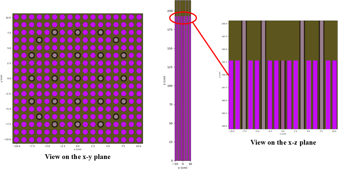
OpenMC geometry colored by material ID shown on the $x$-$y$ and $x$-$z$ planes

Figure 1: OpenMC geometry colored by material ID shown on the $var element = document.getElementById("moose-equation-ff0de1ed-a7d4-45b4-a7ec-3ee768c4049c");katex.render("x", element, {displayMode:false,throwOnError:false});$ - $var element = document.getElementById("moose-equation-8697cb1f-a228-4874-8883-6395a49e44fa");katex.render("y", element, {displayMode:false,throwOnError:false});$ and $var element = document.getElementById("moose-equation-1eb2a2bb-f3b7-42ce-a8dc-06f701b8cc92");katex.render("x", element, {displayMode:false,throwOnError:false});$ - $var element = document.getElementById("moose-equation-8d884f53-06c1-449e-bed4-874a94b01ae9");katex.render("z", element, {displayMode:false,throwOnError:false});$ planes

To generate the XML files needed to run OpenMC, you can run the following:


python make_openmc_model.py

Or you can use the model.xml file that is included in the tutorials/lwr_mgxs directory.

Mesh Mirror for MGXS Generation

Most MGXS workflows store the resulting cross sections in custom libraries for specific deterministic transport codes. Instead, Cardinal determines homogenization volumes using the mesh mirror, and stores the cross sections on the mesh at the end of the OpenMC simulation. This process allows for "transfer" of MGXS between Cardinal and a coupled deterministic code using the multi-app system. This determininstic code coupling enables higher fidelity cross sections generation and recalculation of group properties to account for multi-physics feedback. The input file used to generate this mesh mirror can be found below.

#----------------------------------------------------------------------------------------
# Assembly geometrical information
#----------------------------------------------------------------------------------------
pitch        = 1.26
fuel_height  = 192.78
refl_height  = 21.42
r_fuel       = 0.4095
r_fuel_gap   = 0.4180
r_fuel_clad  = 0.4750
r_guide      = 0.3400
r_guide_clad = 0.5400
#----------------------------------------------------------------------------------------

#----------------------------------------------------------------------------------------
# Meshing parameters
#----------------------------------------------------------------------------------------
NUM_SECTORS              = 4
FUEL_RADIAL_DIVISIONS    = 4
BACKGROUND_DIVISIONS     = 1
AXIAL_DIVISIONS          = 20
#----------------------------------------------------------------------------------------

[Mesh<<<{"href": "../syntax/Mesh/index.html"}>>>]
  [UO2_Pin]
    type = PolygonConcentricCircleMeshGenerator<<<{"description": "This PolygonConcentricCircleMeshGenerator object is designed to mesh a polygon geometry with optional rings centered inside.", "href": "../source/meshgenerators/PolygonConcentricCircleMeshGenerator.html"}>>>
    num_sides<<<{"description": "Number of sides of the polygon."}>>> = 4
    num_sectors_per_side<<<{"description": "Number of azimuthal sectors per polygon side (rotating counterclockwise from top right face)."}>>> = '${NUM_SECTORS} ${NUM_SECTORS} ${NUM_SECTORS} ${NUM_SECTORS}'
    ring_radii<<<{"description": "Radii of major concentric circles (rings)."}>>> = '${r_fuel} ${r_fuel_gap} ${r_fuel_clad}'
    ring_intervals<<<{"description": "Number of radial mesh intervals within each major concentric circle excluding their boundary layers."}>>> = '${FUEL_RADIAL_DIVISIONS} 1 1'
    polygon_size<<<{"description": "Size of the polygon to be generated (given as either apothem or radius depending on polygon_size_style)."}>>> = ${fparse pitch / 2.0}

    ring_block_ids<<<{"description": "Optional customized block ids for each ring geometry block."}>>> = '0 1 2 3'
    ring_block_names<<<{"description": "Optional customized block names for each ring geometry block."}>>> = 'uo2_tri uo2 fuel_gap zr_clad'
    background_block_ids<<<{"description": "Optional customized block id for the background block."}>>> = '9'
    background_block_names<<<{"description": "Optional customized block names for the background block."}>>> = 'water'
    background_intervals<<<{"description": "Number of radial meshing intervals in background region (area between rings and ducts) excluding the background's boundary layers."}>>> = ${BACKGROUND_DIVISIONS}

    flat_side_up<<<{"description": "Whether to rotate the generated polygon mesh to ensure that one flat side faces up."}>>> = true
    quad_center_elements<<<{"description": "Whether the center elements are quad or triangular."}>>> = false
    preserve_volumes<<<{"description": "Volume of concentric circles can be preserved using this function."}>>> = true

    create_outward_interface_boundaries<<<{"description": "Whether the outward interface boundaries are created."}>>> = false
  []
  [Control_Rod_Pin]
    type = PolygonConcentricCircleMeshGenerator<<<{"description": "This PolygonConcentricCircleMeshGenerator object is designed to mesh a polygon geometry with optional rings centered inside.", "href": "../source/meshgenerators/PolygonConcentricCircleMeshGenerator.html"}>>>
    num_sides<<<{"description": "Number of sides of the polygon."}>>> = 4
    num_sectors_per_side<<<{"description": "Number of azimuthal sectors per polygon side (rotating counterclockwise from top right face)."}>>> = '${NUM_SECTORS} ${NUM_SECTORS} ${NUM_SECTORS} ${NUM_SECTORS}'
    ring_radii<<<{"description": "Radii of major concentric circles (rings)."}>>> = '${r_guide} ${r_guide_clad}'
    ring_intervals<<<{"description": "Number of radial mesh intervals within each major concentric circle excluding their boundary layers."}>>> = '${FUEL_RADIAL_DIVISIONS} 1'
    polygon_size<<<{"description": "Size of the polygon to be generated (given as either apothem or radius depending on polygon_size_style)."}>>> = ${fparse pitch / 2.0}

    ring_block_ids<<<{"description": "Optional customized block ids for each ring geometry block."}>>> = '4 5 6'
    ring_block_names<<<{"description": "Optional customized block names for each ring geometry block."}>>> = 'guide_tri guide al_clad'
    background_block_ids<<<{"description": "Optional customized block id for the background block."}>>> = '9'
    background_block_names<<<{"description": "Optional customized block names for the background block."}>>> = 'water'
    background_intervals<<<{"description": "Number of radial meshing intervals in background region (area between rings and ducts) excluding the background's boundary layers."}>>> = ${BACKGROUND_DIVISIONS}

    flat_side_up<<<{"description": "Whether to rotate the generated polygon mesh to ensure that one flat side faces up."}>>> = true
    quad_center_elements<<<{"description": "Whether the center elements are quad or triangular."}>>> = false
    preserve_volumes<<<{"description": "Volume of concentric circles can be preserved using this function."}>>> = true

    create_outward_interface_boundaries<<<{"description": "Whether the outward interface boundaries are created."}>>> = false
  []
  [Fission_Chamber_Pin]
    type = PolygonConcentricCircleMeshGenerator<<<{"description": "This PolygonConcentricCircleMeshGenerator object is designed to mesh a polygon geometry with optional rings centered inside.", "href": "../source/meshgenerators/PolygonConcentricCircleMeshGenerator.html"}>>>
    num_sides<<<{"description": "Number of sides of the polygon."}>>> = 4
    num_sectors_per_side<<<{"description": "Number of azimuthal sectors per polygon side (rotating counterclockwise from top right face)."}>>> = '${NUM_SECTORS} ${NUM_SECTORS} ${NUM_SECTORS} ${NUM_SECTORS}'
    ring_radii<<<{"description": "Radii of major concentric circles (rings)."}>>> = '${r_guide} ${r_guide_clad}'
    ring_intervals<<<{"description": "Number of radial mesh intervals within each major concentric circle excluding their boundary layers."}>>> = '${FUEL_RADIAL_DIVISIONS} 1'
    polygon_size<<<{"description": "Size of the polygon to be generated (given as either apothem or radius depending on polygon_size_style)."}>>> = ${fparse pitch / 2.0}

    ring_block_ids<<<{"description": "Optional customized block ids for each ring geometry block."}>>> = '7 8 6'
    ring_block_names<<<{"description": "Optional customized block names for each ring geometry block."}>>> = 'fission_tri fission al_clad'
    background_block_ids<<<{"description": "Optional customized block id for the background block."}>>> = '9'
    background_block_names<<<{"description": "Optional customized block names for the background block."}>>> = 'water'
    background_intervals<<<{"description": "Number of radial meshing intervals in background region (area between rings and ducts) excluding the background's boundary layers."}>>> = ${BACKGROUND_DIVISIONS}

    flat_side_up<<<{"description": "Whether to rotate the generated polygon mesh to ensure that one flat side faces up."}>>> = true
    quad_center_elements<<<{"description": "Whether the center elements are quad or triangular."}>>> = false
    preserve_volumes<<<{"description": "Volume of concentric circles can be preserved using this function."}>>> = true

    create_outward_interface_boundaries<<<{"description": "Whether the outward interface boundaries are created."}>>> = false
  []
  [UO2_Assembly]
    type = PatternedCartesianMeshGenerator<<<{"description": "This PatternedCartesianMeshGenerator source code assembles square meshes into a square grid and optionally forces the outer boundary to be square and/or adds a duct.", "href": "../source/meshgenerators/PatternedCartesianMeshGenerator.html"}>>>
    inputs<<<{"description": "The names of the meshes forming the pattern."}>>> = 'UO2_Pin Control_Rod_Pin Fission_Chamber_Pin'
    pattern<<<{"description": "A two-dimensional cartesian (square-shaped) array starting with the upper-left corner.It is composed of indexes into the inputs vector"}>>> = '0 0 0 0 0 0 0 0 0 0 0 0 0 0 0 0 0;
               0 0 0 0 0 0 0 0 0 0 0 0 0 0 0 0 0;
               0 0 0 0 0 1 0 0 1 0 0 1 0 0 0 0 0;
               0 0 0 1 0 0 0 0 0 0 0 0 0 1 0 0 0;
               0 0 0 0 0 0 0 0 0 0 0 0 0 0 0 0 0;
               0 0 1 0 0 1 0 0 1 0 0 1 0 0 1 0 0;
               0 0 0 0 0 0 0 0 0 0 0 0 0 0 0 0 0;
               0 0 0 0 0 0 0 0 0 0 0 0 0 0 0 0 0;
               0 0 1 0 0 1 0 0 2 0 0 1 0 0 1 0 0;
               0 0 0 0 0 0 0 0 0 0 0 0 0 0 0 0 0;
               0 0 0 0 0 0 0 0 0 0 0 0 0 0 0 0 0;
               0 0 1 0 0 1 0 0 1 0 0 1 0 0 1 0 0;
               0 0 0 0 0 0 0 0 0 0 0 0 0 0 0 0 0;
               0 0 0 1 0 0 0 0 0 0 0 0 0 1 0 0 0;
               0 0 0 0 0 1 0 0 1 0 0 1 0 0 0 0 0;
               0 0 0 0 0 0 0 0 0 0 0 0 0 0 0 0 0;
               0 0 0 0 0 0 0 0 0 0 0 0 0 0 0 0 0'

    pattern_boundary<<<{"description": "The boundary shape of the patterned mesh."}>>> = 'none'

    assign_type<<<{"description": "List of integer ID assignment types"}>>> = 'cell'
    id_name<<<{"description": "List of extra integer ID set names"}>>> = 'pin_id'
    generate_core_metadata<<<{"description": "A Boolean parameter that controls whether the core related metadata is generated for other MOOSE objects such as 'MultiControlDrumFunction' or not."}>>> = false
  []
  [To_Origin]
    type = TransformGenerator<<<{"description": "Applies a linear transform to the entire mesh.", "href": "../source/meshgenerators/TransformGenerator.html"}>>>
    input<<<{"description": "The mesh we want to modify"}>>> = 'UO2_Assembly'
    transform<<<{"description": "The type of transformation to perform (TRANSLATE, TRANSLATE_CENTER_ORIGIN, TRANSLATE_MIN_ORIGIN, ROTATE, SCALE)"}>>> = TRANSLATE_CENTER_ORIGIN
  []
  [3D_Core]
    type = AdvancedExtruderGenerator<<<{"description": "Extrudes a 1D mesh into 2D, or a 2D mesh into 3D, can have a variable height for each elevation, variable number of layers within each elevation, variable growth factors of axial element sizes within each elevation and remap subdomain_ids, boundary_ids and element extra integers within each elevation as well as interface boundaries between neighboring elevation layers.", "href": "../source/meshgenerators/AdvancedExtruderGenerator.html"}>>>
    input<<<{"description": "The mesh to extrude"}>>> = 'To_Origin'
    heights<<<{"description": "The height of each elevation"}>>> = '${fparse fuel_height} ${fparse refl_height}'
    num_layers<<<{"description": "The number of layers for each elevation - must be num_elevations in length!"}>>> = '${AXIAL_DIVISIONS} 2'
    subdomain_swaps<<<{"description": "For each row, every two entries are interpreted as a pair of 'from' and 'to' to remap the subdomains for that elevation"}>>> = ';
                       0 10 1 9 2 9 3 9'
    direction<<<{"description": "A vector that points in the direction to extrude (note, this will be normalized internally - so don't worry about it here)"}>>> = '0.0 0.0 1.0'
  []
  [Rename]
    type = RenameBlockGenerator<<<{"description": "Changes the block IDs and/or block names for a given set of blocks defined by either block ID or block name. The changes are independent of ordering. The merging of blocks is supported.", "href": "../source/meshgenerators/RenameBlockGenerator.html"}>>>
    input<<<{"description": "The mesh we want to modify"}>>> = '3D_Core'
    old_block<<<{"description": "Elements with these block ID(s)/name(s) will be given the new block information specified in 'new_block'"}>>> = '10'
    new_block<<<{"description": "The new block ID(s)/name(s) to be given by the elements defined in 'old_block'."}>>> = 'water_tri'
  []
[]

The mesh is similar to the mesh generated in the AMR tutorial with a few key differences to accommodate a coupled deterministic transport code. We set NUM_SECTORS and FUEL_RADIAL_DIVISIONS to 4 to increase the radial fidelity of of each pin. The increased discretization is necessary for deterministic calculations as these regions have strong gradients due to absorption in the fuel and control rods. We also avoid deleting the gap blocks and extruded the mesh an additional 21.42 cm to cover the reflector. These changes are necessary to preserve mesh connectivity for deterministic transport solvers using these cross sections, and to ensure we generate cross sections for the reflector above the core.

  [3D_Core]
    type = AdvancedExtruderGenerator
    input = 'To_Origin'
    heights = '${fparse fuel_height} ${fparse refl_height}'
    num_layers = '${AXIAL_DIVISIONS} 2'
    subdomain_swaps = ';
                       0 10 1 9 2 9 3 9'
    direction = '0.0 0.0 1.0'
  []

The input mesh Cardinal will use to store cell tally results on (mesh_in.e) can be generated by running the command below. The resulting mesh can be found in Figure 2; we note that this mesh is substantially finer than a conventional Cardinal mesh mirror to adequately capture spatial gradients in the deterministic solver.


cardinal-opt -i mesh.i --mesh-only

The mesh mirror used for computing and storing [!ac](MGXS), shown with an isometric view and sliced on the $x-y$ plane

Figure 2: The mesh mirror used for computing and storing MGXS, shown with an isometric view and sliced on the $var element = document.getElementById("moose-equation-c4be4271-b5d2-4a54-a29f-7d35ae8a3e11");katex.render("x-y", element, {displayMode:false,throwOnError:false});$ plane

Neutronics Input File

The neutronics calculation is performed over the entire assembly by OpenMC and the wrapping of the OpenMC results in MOOSE is performed in openmc_mgxs.i. We begin by defining the mesh (generated in the previous step) used by Cardinal to determine which cell tallies should be constructed for MGXS generation:

[Mesh<<<{"href": "../syntax/Mesh/index.html"}>>>]
  [file]
    type = FileMeshGenerator<<<{"description": "Read a mesh from a file.", "href": "../source/meshgenerators/FileMeshGenerator.html"}>>>
    file<<<{"description": "The filename to read."}>>> = mesh_in.e
  []
[]

Afterwards, we add two auxvariables and auxkernels for post-processing the cross sections – we use these to compute the scattering ratio (the sum of scattering cross sections divided by the total cross section) in each energy group. Physically, the scattering ratio for each group should be less than or equal to one; scattering ratios larger than one may result in non-convergence of the deterministic solver or convergence to incorrect results. Note that we did not delete the gap blocks in the mesh, but we are block restricting the auxkernels and auxvariables such that they are not computed over the gap region (block 2). This is necessary as the gaps do not receive any tally hits in OpenMC. Therefore, the cross sections will be zero resulting in a divide by zero when computing scattering ratios.

[AuxVariables<<<{"href": "../syntax/AuxVariables/index.html"}>>>]
  [scatter_ratio_g1]
    type = MooseVariable<<<{"description": "Represents standard field variables, e.g. Lagrange, Hermite, or non-constant Monomials", "href": "../source/variables/MooseVariable.html"}>>>
    family<<<{"description": "Specifies the family of FE shape functions to use for this variable"}>>> = MONOMIAL
    order<<<{"description": "Specifies the order of the FE shape function to use for this variable (additional orders not listed are allowed)"}>>> = CONSTANT
    block<<<{"description": "The list of blocks (ids or names) that this object will be applied"}>>> = '0 1 3 4 5 6 7 8 9 10'
  []
  [scatter_ratio_g2]
    type = MooseVariable<<<{"description": "Represents standard field variables, e.g. Lagrange, Hermite, or non-constant Monomials", "href": "../source/variables/MooseVariable.html"}>>>
    family<<<{"description": "Specifies the family of FE shape functions to use for this variable"}>>> = MONOMIAL
    order<<<{"description": "Specifies the order of the FE shape function to use for this variable (additional orders not listed are allowed)"}>>> = CONSTANT
    block<<<{"description": "The list of blocks (ids or names) that this object will be applied"}>>> = '0 1 3 4 5 6 7 8 9 10'
  []
[]

[AuxKernels<<<{"href": "../syntax/AuxKernels/index.html"}>>>]
  [comp_scatter_ratio_g1]
    type = ParsedAux<<<{"description": "Sets a field variable value to the evaluation of a parsed expression.", "href": "../source/auxkernels/ParsedAux.html"}>>>
    variable<<<{"description": "The name of the variable that this object applies to"}>>> = scatter_ratio_g1
    coupled_variables<<<{"description": "Vector of coupled variable names"}>>> = 'total_xs_g1 scatter_xs_g1_gp1_l0 scatter_xs_g1_gp2_l0'
    expression<<<{"description": "Parsed function expression to compute"}>>> = '(scatter_xs_g1_gp1_l0 + scatter_xs_g1_gp2_l0) / total_xs_g1'
    block<<<{"description": "The list of blocks (ids or names) that this object will be applied"}>>> = '0 1 3 4 5 6 7 8 9 10'
  []
  [comp_scatter_ratio_g2]
    type = ParsedAux<<<{"description": "Sets a field variable value to the evaluation of a parsed expression.", "href": "../source/auxkernels/ParsedAux.html"}>>>
    variable<<<{"description": "The name of the variable that this object applies to"}>>> = scatter_ratio_g2
    coupled_variables<<<{"description": "Vector of coupled variable names"}>>> = 'total_xs_g2 scatter_xs_g2_gp1_l0 scatter_xs_g2_gp2_l0'
    expression<<<{"description": "Parsed function expression to compute"}>>> = '(scatter_xs_g2_gp1_l0 + scatter_xs_g2_gp2_l0) / total_xs_g2'
    block<<<{"description": "The list of blocks (ids or names) that this object will be applied"}>>> = '0 1 3 4 5 6 7 8 9 10'
  []
[]

Next, the Problem block (with an OpenMCCellAverageProblem) describes the syntax necessary to replace the normal MOOSE finite element calculation with an OpenMC neutronics solve. We select cell_level = 1 to ensure that we generate our cell to element mapping for an OpenMC geometry depth one lower than the root universe. This will result in a distributed cell tally for each unique geometric region in the LWR lattice, as opposed to the entire lattice (which is what would happen with cell_level = 0, because the lattice is filled inside another cell which forms the root universe). We then specify the number of particles, the number of inactive batches, and the total number of batches.

[Problem<<<{"href": "../syntax/Problem/index.html"}>>>]
  type = OpenMCCellAverageProblem
  # Since we're generating multi-group cross sections the value
  # of power chosen is arbitrary.
  power = 1.0
  # We set the cell level to 1 to ensure we get multi-group cross
  # sections for each unique cell in the lattice.
  cell_level = 1

  verbose = true
  particles = 10000
  inactive_batches = 50
  batches = 1000

  # The MGXS block is adding fission heating, so we set the source
  # rate normalization to 'kappa_fission'.
  source_rate_normalization = 'kappa_fission'
[]

After specifying the basic problem settings, we move on to setting up the MGXS parameters with the MGXS block. We specify a distributed cell tally should be used as the MGXS homogenization domain with tally_type = cell and the CASMO 2 group structure as the energy group boundaries. We then select particle = neutron to set the particle filter to use when computing cross sections, which is useful when OpenMC is performing coupled neutron-photon transport. We then specify estimator = 'analog', which is required when computing scattering cross sections and the fission spectra. For the same reasons as the auxkernels added for post-processing, we block restrict the MGXS such that they are not computed on the gap region. Finally, we select the MGXS that we wish to compute. This includes total cross sections (always computed), scattering matrix cross sections (enabled by default), nu-fission cross sections (add_fission = true), fission chi spectra (add_fission = true), and fission heating cross sections (add_fission_heating = true). Note, other cross sections or group properties can be computed; an exhaustive list of the options can be found in the documentation for the MGXS block. We choose to disable the transport correction (transport_correction = false) for the scattering cross sections to avoid pushing the scattering ratio over unity, which can occur when there aren't enough particles scoring to higher order scattering moments.

[Problem<<<{"href": "../syntax/Problem/index.html"}>>>/MGXS<<<{"href": "../syntax/Problem/MGXS/index.html"}>>>]
  tally_type<<<{"description": "The type of spatial tally to use"}>>> = cell
  group_structure<<<{"description": "The energy group structure to use from a list of popular group structures."}>>> = CASMO_2
  particle<<<{"description": "The particle to filter for. At present cross sections can only be generated for neutrons or photons, if 'electron' or 'positron' are selected an error will be thrown."}>>> = neutron
  estimator<<<{"description": "The type of estimator to use with the tallies added for MGXS generation. This is not applied to scattering / fission scores as the filters applied to those scores only support analog estimators."}>>> = analog
  block<<<{"description": "The list of block ids (SubdomainID) to which this action will be applied"}>>> = '0 1 3 4 5 6 7 8 9 10'

  add_fission<<<{"description": "Whether or not fission multi-group cross sections (neutron production and the discrete chi spectrum) should be generated."}>>> = true

  add_fission_heating<<<{"description": "Whether or not per-group fission heating (kappa-fission) values should be generated."}>>> = true

  transport_correction<<<{"description": "Whether the in-group scattering cross section should include a P0 transport correction or not."}>>> = false
[]

Since we've selected add_fission_heating = true, we don't need to add other heating tallies for normalization purposes – we can set source_rate_normalization = 'kappa_fission' in the Problem block. A steady-state executioner is selected as OpenMC will run a single criticality calculation. We then select exodus output which will occur on the end of the simulation.

[Executioner<<<{"href": "../syntax/Executioner/index.html"}>>>]
  type = Steady
[]

[Outputs<<<{"href": "../syntax/Outputs/index.html"}>>>]
  exodus<<<{"description": "Output the results using the default settings for Exodus output."}>>> = true
  execute_on<<<{"description": "The list of flag(s) indicating when this object should be executed. For a description of each flag, see https://mooseframework.inl.gov/source/interfaces/SetupInterface.html."}>>> = 'TIMESTEP_END'
[]

Execution and Postprocessing

To run the wrapped neutronics calculation,


mpiexec -np 2 cardinal-opt -i openmc.i --n-threads=4

This will run OpenMC with 2 MPI ranks with 4 OpenMP threads per rank. To run the simulation faster, you can increase the parallel processes/threads, or simply decrease the number of particles used in OpenMC. When the simulation is complete, you will have created openmc_out.e, an Exodus mesh with the computed cross sections. In the console output, you should see the following tally list:


---------------------------------------------------------------------------------
|          Tally Name          |  Tally Score  |         AuxVariable(s)         |
---------------------------------------------------------------------------------
| MGXS_CellTally_Total_Flux    | total         | mgxs_total_g2_neutron          |
|                              |               | mgxs_total_g1_neutron          |
|                              | flux          | mgxs_flux_g2_neutron           |
|                              |               | mgxs_flux_g1_neutron           |
| MGXS_CellTally_Scatter       | nu-scatter    | mgxs_scatter_g2_gp2_l0_neutron |
|                              |               | mgxs_scatter_g2_gp1_l0_neutron |
|                              |               | mgxs_scatter_g1_gp2_l0_neutron |
|                              |               | mgxs_scatter_g1_gp1_l0_neutron |
| MGXS_CellTally_Fission       | nu-fission    | mgxs_fission_g2_gp2_neutron    |
|                              |               | mgxs_fission_g2_gp1_neutron    |
|                              |               | mgxs_fission_g1_gp2_neutron    |
|                              |               | mgxs_fission_g1_gp1_neutron    |
| MGXS_CellTally_Kappa_Fission | kappa-fission | mgxs_kappa_fission_g2_neutron  |
|                              |               | mgxs_kappa_fission_g1_neutron  |
---------------------------------------------------------------------------------

Each of these tallies are automatically applied to the cells discovered by Cardinal when generating the cell to element mapping. The generated cross sections for the fuel can be found in Figure 3, where we can see the importance of accurately capturing spatial and spectral effects when generating group constants. The fast neutron production cross sections for the corner pins of the LWR assembly are larger then the central pins due to spatial shielding effects. The thermal neutron production cross section increases in the region between the center and periphery of the assembly due to an increase in moderation. Additionally, a depression in the thermal neutron production cross section can also be seen in the fuel pins close to the inserted control rods.

The generated [!ac](MGXS) at the core centerline. Left: $\chi_{g}$. Middle: $\nu\Sigma_{f,g}$. Right: $\kappa\Sigma_{f,g}$.

Figure 3: The generated MGXS at the core centerline. Left: $var element = document.getElementById("moose-equation-14a70f4c-d16b-4ba3-b618-a31c20ed7e74");katex.render("\\chi_{g}", element, {displayMode:false,throwOnError:false});$ . Middle: $var element = document.getElementById("moose-equation-ed40b839-da71-43df-9fa0-35690e81aaf5");katex.render("\\nu\\Sigma_{f,g}", element, {displayMode:false,throwOnError:false});$ . Right: $var element = document.getElementById("moose-equation-517d658d-0cd7-4177-885b-be5d7b7ba7d8");katex.render("\\kappa\\Sigma_{f,g}", element, {displayMode:false,throwOnError:false});$ .

The group-wise total cross section and scattering ratio for all materials at the core centerline can be found in Figure 4. Spatial trends are difficult to pick out due to the order-of-magnitude difference between MGXS for the different materials. However, we see the control rods are the strongest absorbers in both the fast and thermal range. The borated water coolant has a very large scattering ratio in both the fast and thermal groups, showcasing the effectiveness of water as a neutron moderator.

The generated [!ac](MGXS) at the core centerline. Left: $\Sigma_{t,g}$. Right: $\Sigma_{s,g} / \Sigma_{t,g}$.

Figure 4: The generated MGXS at the core centerline. Left: $var element = document.getElementById("moose-equation-1aba2ba9-4c47-4122-bea7-fb768429873b");katex.render("\\Sigma_{t,g}", element, {displayMode:false,throwOnError:false});$ . Right: $var element = document.getElementById("moose-equation-d668493f-c912-461c-85c7-7a6f81addb08");katex.render("\\Sigma_{s,g} / \\Sigma_{t,g}", element, {displayMode:false,throwOnError:false});$ .

Results in a Deterministic Code

While not a capability available in Cardinal, we take these MGXS and use them as an input in a deterministic solver to showcase the end result of a standard two-step calculation. The fast and thermal fluxes from the discrete-ordinates code Gnat (Sawatzky and Atkinson (2024)) using these cross sections can be found in Figure 5 and Figure 6. The predicted continuous-energy value of $var element = document.getElementById("moose-equation-35bb926b-4e9a-4dc3-b74a-8ae81bfb6d72");katex.render("k_{eff}", element, {displayMode:false,throwOnError:false});$ from Cardinal-OpenMC is $var element = document.getElementById("moose-equation-71e4a7d5-e18b-42cb-917c-db988ed39c86");katex.render("0.64684", element, {displayMode:false,throwOnError:false});$ . Gnat (using 200 directions per energy group) obtains a multi-group $var element = document.getElementById("moose-equation-a7cf31e6-6cf0-4c7a-ba17-f13537d6a286");katex.render("k_{eff}", element, {displayMode:false,throwOnError:false});$ of $var element = document.getElementById("moose-equation-cba65f38-2087-4100-b9d6-43cfef84186c");katex.render("0.64372", element, {displayMode:false,throwOnError:false});$ , yielding $var element = document.getElementById("moose-equation-3cf4d89b-3dab-4243-8246-57ca87eb3dab");katex.render("\\Delta k_{eff} = 312", element, {displayMode:false,throwOnError:false});$ pcm. There is likely some amount of cancellation of error in the deterministic result, evidenced by the surprisingly good agreement obtained without using transport-corrected scattering cross sections. However, we believe these results showcase the value of this automated workflow for computing spatially-varying cross sections for deterministic transport calculations.

Group 1 (fast) fluxes from Gnat using the generated [!ac](MGXS). Fluxes are normalized such that the integral over all space and energy is unity.

Figure 5: Group 1 (fast) fluxes from Gnat using the generated MGXS. Fluxes are normalized such that the integral over all space and energy is unity.

Group 2 (thermal) fluxes from Gnat using the generated [!ac](MGXS). Fluxes are normalized such that the integral over all space and energy is unity.

Figure 6: Group 2 (thermal) fluxes from Gnat using the generated MGXS. Fluxes are normalized such that the integral over all space and energy is unity.

References

S. Cathalau, J. C. Lefebvre, and J. P. West. Proposal for a Second Stage of the Benchmark on Power Distributions within Assemblies. Technical Report NEA/NSC/DOC(96)2, Organisation for Economic Cooperation and Development, Nuclear Energy Agency, 1996. URL: https://www.oecd-nea.org/upload/docs/application/pdf/2020-01/nsc-doc96-02-rev2.pdf.

@TechReport{c5g7_materials,
    author = "Cathalau, S. and Lefebvre, J. C. and West, J. P.",
    title = "{Proposal for a Second Stage of the Benchmark on Power Distributions within Assemblies}",
    institution = "Organisation for Economic Cooperation and Development, Nuclear Energy Agency",
    year = "1996",
    number = "NEA/NSC/DOC(96)2",
    url = "https://www.oecd-nea.org/upload/docs/application/pdf/2020-01/nsc-doc96-02-rev2.pdf"
}

K. Sawatzky and K. D. Atkinson. Verification of a CARIBOU-OpenMC Workflow for the Analysis of HTGR-Like Systems Using the Proposed Ontario Tech Subcritical Assembly. In Proceedings of PHYSOR. 2024.

@InProceedings{gnat_1,
    author = "Sawatzky, K. and Atkinson, K. D.",
    title = "{Verification of a CARIBOU-OpenMC Workflow for the Analysis of HTGR-Like Systems Using the Proposed Ontario Tech Subcritical Assembly}",
    booktitle = "{Proceedings of PHYSOR}",
    year = "2024"
}

M.A. Smith, E.E. Lewis, and Byung-Chan Na. Benchmark on Deterministic 3-D MOX Fuel Assembly Transport Calculations without Spatial Homogenization. Progress in Nuclear Energy, 48(5):383–393, 2006. doi:https://doi.org/10.1016/j.pnucene.2006.01.002.

@article{c5g7,
    author = "Smith, M.A. and Lewis, E.E. and Na, Byung-Chan",
    title = "{Benchmark on Deterministic 3-D MOX Fuel Assembly Transport Calculations without Spatial Homogenization}",
    journal = "{Progress in Nuclear Energy}",
    volume = "48",
    number = "5",
    pages = "383-393",
    year = "2006",
    doi = "https://doi.org/10.1016/j.pnucene.2006.01.002"
}

(tutorials/lwr_amr/make_openmc_model.py)

#********************************************************************/
#*                  SOFTWARE COPYRIGHT NOTIFICATION                 */
#*                             Cardinal                             */
#*                                                                  */
#*                  (c) 2021 UChicago Argonne, LLC                  */
#*                        ALL RIGHTS RESERVED                       */
#*                                                                  */
#*                 Prepared by UChicago Argonne, LLC                */
#*               Under Contract No. DE-AC02-06CH11357               */
#*                With the U. S. Department of Energy               */
#*                                                                  */
#*             Prepared by Battelle Energy Alliance, LLC            */
#*               Under Contract No. DE-AC07-05ID14517               */
#*                With the U. S. Department of Energy               */
#*                                                                  */
#*                 See LICENSE for full restrictions                */
#********************************************************************/

#--------------------------------------------------------------------------------------------------------------------------#
# This is based on the C5G7 reactor physics benchmark problem extension case as described in:                              #
# "Benchmark on Deterministic Transport Calculations Without Spatial Homogenisation: MOX Fuel Assembly 3-D Extension Case" #
# [NEA/NSC/DOC(2005)16]                                                                                                    #
# https://www.oecd-nea.org/upload/docs/application/pdf/2019-12/nsc-doc2005-16.pdf                                          #                                                                                                                     #
#                                                                                                                          #
# The original C5G7 benchmark is defined with multi-group cross sections. To account for                                   #
# continuous energy spectral effects, we chose to use the material properties provided in:                                 #
# "Proposal for a Second Stage of the Benchmark on Power Distributions Within Assemblies"                                  #
# [NEA/NSC/DOC(96)2]                                                                                                       #
# https://www.oecd-nea.org/upload/docs/application/pdf/2020-01/nsc-doc96-02-rev2.pdf                                       #
#--------------------------------------------------------------------------------------------------------------------------#

import openmc
import numpy as np
import openmc.universe
from argparse import ArgumentParser

ap = ArgumentParser()
ap.add_argument('-n', dest='n_axial', type=int, default=1,
                help='Number of axial core divisions')
args = ap.parse_args()

#--------------------------------------------------------------------------------------------------------------------------#
# Some geometric properties that can be modified to change the model.
## The radius of a fuel pin (same for all pin types).
r_fuel = 0.4095

## The thickness of the fuel-clad gap.
t_f_c_gap = 0.0085

## The thickness of the Zr fuel pin cladding.
t_zr_clad = 0.057

## The radius of the control rod guide tubes and the fission chambers.
r_guide = 0.3400

## The thickness of the guide tube / fission chamber Al cladding.
t_al_clad = 0.2

## The pitch of a single lattice element.
pitch = 1.26

## The height of the fuel assemblies from the axial midplane.
core_height = 192.78

## The thickness of the water reflector around the fuel assemblies, both axial and radial.
reflector_t = 21.42

# Some discretization parameters.
core_axial_slices = args.n_axial
#--------------------------------------------------------------------------------------------------------------------------#

#--------------------------------------------------------------------------------------------------------------------------#
# Material definitions.

## Fuel region: UO2 at ~1% enriched.
uo2_comp = 1.0e24 * np.array([8.65e-4, 2.225e-2, 4.622e-2])
uo2_frac = uo2_comp / np.sum(uo2_comp)
uo2 = openmc.Material(name = 'UO2 Fuel', temperature = 293.15)
uo2.add_nuclide('U235', uo2_frac[0], percent_type = 'ao')
uo2.add_nuclide('U238', uo2_frac[1], percent_type = 'ao')
uo2.add_element('O', uo2_frac[2], percent_type = 'ao')
uo2.set_density('atom/cm3', np.sum(uo2_comp))

## Control rod meat: assumed to be B-10 carbide (B4C).
bc4 = openmc.Material(name = 'Control Rod Meat', temperature = 293.15)
bc4.add_element('B', 4.0, percent_type = 'ao')
bc4.add_element('C', 1.0, percent_type = 'ao')
bc4.set_density('atom/cm3', 2.75e23)

## Moderator and coolant, boronated water.
h2o_comp = 1.0e24 * np.array([3.35e-2, 2.78e-5])
h2o_frac = h2o_comp / np.sum(h2o_comp)
h2o = openmc.Material(name = 'H2O Moderator', temperature = 293.15)
h2o.add_element('H', 2.0 * h2o_frac[0], percent_type = 'ao')
h2o.add_element('O', h2o_frac[0], percent_type = 'ao')
h2o.add_element('B', h2o_frac[1], percent_type = 'ao')
h2o.set_density('atom/cm3', np.sum(h2o_comp))
h2o.add_s_alpha_beta('c_H_in_H2O')

## Fission chamber.
fiss_comp = 1.0e24 * np.array([3.35e-2, 2.78e-5, 1.0e-8])
fiss_frac = fiss_comp / np.sum(fiss_comp)
fiss = openmc.Material(name = 'Fission Chamber', temperature = 293.15)
fiss.add_element('H', 2.0 * fiss_frac[0], percent_type = 'ao')
fiss.add_element('O', fiss_frac[0], percent_type = 'ao')
fiss.add_element('B', fiss_frac[1], percent_type = 'ao')
fiss.add_nuclide('U235', fiss_frac[2], percent_type = 'ao')
fiss.set_density('atom/cm3', np.sum(fiss_comp))
fiss.add_s_alpha_beta('c_H_in_H2O')

## Zr clad.
zr = openmc.Material(name = 'Zr Cladding', temperature = 293.15)
zr.add_element('Zr', 1.0, percent_type = 'ao')
zr.set_density('atom/cm3', 1.0e24 * 4.30e-2)

## Al clad.
al = openmc.Material(name = 'Al Cladding', temperature = 293.15)
al.add_element('Al', 1.0, percent_type = 'ao')
al.set_density('atom/cm3', 1.0e24 * 6.0e-2)
#--------------------------------------------------------------------------------------------------------------------------#

#--------------------------------------------------------------------------------------------------------------------------#
# Geometry definitions.
## Fuel first
### The entire UO2 pincell.
fuel_pin_or = openmc.ZCylinder(r = r_fuel)
fuel_gap_1_or = openmc.ZCylinder(r = r_fuel + t_f_c_gap)
fuel_zr_or = openmc.ZCylinder(r = r_fuel + t_f_c_gap + t_zr_clad)
fuel_bb = openmc.model.RectangularPrism(width = pitch, height = pitch)

gap_1_cell_4 = openmc.Cell(name = 'UO2 Pin Gap 1')
gap_1_cell_4.region = +fuel_pin_or & -fuel_gap_1_or
zr_clad_cell_4 = openmc.Cell(name = 'UO2 Pin Zr Clad')
zr_clad_cell_4.region = +fuel_gap_1_or & -fuel_zr_or
zr_clad_cell_4.fill = zr
h2o_bb_cell_4 = openmc.Cell(name = 'UO2 Pin Water Bounding Box')
h2o_bb_cell_4.region = +fuel_zr_or & -fuel_bb
h2o_bb_cell_4.fill = h2o

uo2_fuel_cell = openmc.Cell(name = 'UO2 Fuel Pin')
uo2_fuel_cell.region = -fuel_pin_or
uo2_fuel_cell.fill = uo2
uo2_u = openmc.Universe(cells=[uo2_fuel_cell, gap_1_cell_4, zr_clad_cell_4, h2o_bb_cell_4])

## Guide tube and fission chamber next.
### Common primitives for defining both.
tube_fill_or = openmc.ZCylinder(r = r_guide)
tube_clad_or = openmc.ZCylinder(r = r_guide + t_al_clad)

tube_clad_cell_1 = openmc.Cell(name = 'Control Rod Cladding')
tube_clad_cell_1.region = +tube_fill_or & -tube_clad_or
tube_clad_cell_1.fill = al

tube_clad_cell_2 = openmc.Cell(name = 'Fission Chamber Cladding')
tube_clad_cell_2.region = +tube_fill_or & -tube_clad_or
tube_clad_cell_2.fill = al

guide_tube_h2o_bb_cell_1 = openmc.Cell(name = 'Guide Tube Water Bounding Box')
guide_tube_h2o_bb_cell_1.region = +tube_clad_or & -fuel_bb
guide_tube_h2o_bb_cell_1.fill = h2o

guide_tube_h2o_bb_cell_2 = openmc.Cell(name = 'Fission Chamber Water Bounding Box')
guide_tube_h2o_bb_cell_2.region = +tube_clad_or & -fuel_bb
guide_tube_h2o_bb_cell_2.fill = h2o

### The guide tube.
rod_fill_cell = openmc.Cell(name = 'Control Rod Meat')
rod_fill_cell.region = -tube_fill_or
rod_fill_cell.fill = bc4
rod_u = openmc.Universe(cells=[rod_fill_cell, tube_clad_cell_1, guide_tube_h2o_bb_cell_1])

### The fission chamber.
fission_chamber_cell = openmc.Cell(name = 'Fission Chamber')
fission_chamber_cell.region = -tube_fill_or
fission_chamber_cell.fill = fiss
fis_u = openmc.Universe(cells=[fission_chamber_cell, tube_clad_cell_2, guide_tube_h2o_bb_cell_2])

### An empty water cell to build the upper reflector.
water_cell = openmc.Cell(name = 'Reflector Water')
water_cell.region = -fuel_bb
water_cell.fill = h2o
wat_u = openmc.Universe(cells=[water_cell])

## The assembly.
assembly_bb = openmc.model.RectangularPrism(origin = (0.0, 0.0), width = 16.9 * pitch, height = 16.9 * pitch, boundary_type = 'reflective')

### UO2 fueled assembly.
uo2_assembly_cells = [
  [uo2_u, uo2_u, uo2_u, uo2_u, uo2_u, uo2_u, uo2_u, uo2_u, uo2_u, uo2_u, uo2_u, uo2_u, uo2_u, uo2_u, uo2_u, uo2_u, uo2_u], # 1
  [uo2_u, uo2_u, uo2_u, uo2_u, uo2_u, uo2_u, uo2_u, uo2_u, uo2_u, uo2_u, uo2_u, uo2_u, uo2_u, uo2_u, uo2_u, uo2_u, uo2_u], # 2
  [uo2_u, uo2_u, uo2_u, uo2_u, uo2_u, rod_u, uo2_u, uo2_u, rod_u, uo2_u, uo2_u, rod_u, uo2_u, uo2_u, uo2_u, uo2_u, uo2_u], # 3
  [uo2_u, uo2_u, uo2_u, rod_u, uo2_u, uo2_u, uo2_u, uo2_u, uo2_u, uo2_u, uo2_u, uo2_u, uo2_u, rod_u, uo2_u, uo2_u, uo2_u], # 4
  [uo2_u, uo2_u, uo2_u, uo2_u, uo2_u, uo2_u, uo2_u, uo2_u, uo2_u, uo2_u, uo2_u, uo2_u, uo2_u, uo2_u, uo2_u, uo2_u, uo2_u], # 5
  [uo2_u, uo2_u, rod_u, uo2_u, uo2_u, rod_u, uo2_u, uo2_u, rod_u, uo2_u, uo2_u, rod_u, uo2_u, uo2_u, rod_u, uo2_u, uo2_u], # 6
  [uo2_u, uo2_u, uo2_u, uo2_u, uo2_u, uo2_u, uo2_u, uo2_u, uo2_u, uo2_u, uo2_u, uo2_u, uo2_u, uo2_u, uo2_u, uo2_u, uo2_u], # 7
  [uo2_u, uo2_u, uo2_u, uo2_u, uo2_u, uo2_u, uo2_u, uo2_u, uo2_u, uo2_u, uo2_u, uo2_u, uo2_u, uo2_u, uo2_u, uo2_u, uo2_u], # 8
  [uo2_u, uo2_u, rod_u, uo2_u, uo2_u, rod_u, uo2_u, uo2_u, fis_u, uo2_u, uo2_u, rod_u, uo2_u, uo2_u, rod_u, uo2_u, uo2_u], # 9
  [uo2_u, uo2_u, uo2_u, uo2_u, uo2_u, uo2_u, uo2_u, uo2_u, uo2_u, uo2_u, uo2_u, uo2_u, uo2_u, uo2_u, uo2_u, uo2_u, uo2_u], # 10
  [uo2_u, uo2_u, uo2_u, uo2_u, uo2_u, uo2_u, uo2_u, uo2_u, uo2_u, uo2_u, uo2_u, uo2_u, uo2_u, uo2_u, uo2_u, uo2_u, uo2_u], # 11
  [uo2_u, uo2_u, rod_u, uo2_u, uo2_u, rod_u, uo2_u, uo2_u, rod_u, uo2_u, uo2_u, rod_u, uo2_u, uo2_u, rod_u, uo2_u, uo2_u], # 12
  [uo2_u, uo2_u, uo2_u, uo2_u, uo2_u, uo2_u, uo2_u, uo2_u, uo2_u, uo2_u, uo2_u, uo2_u, uo2_u, uo2_u, uo2_u, uo2_u, uo2_u], # 13
  [uo2_u, uo2_u, uo2_u, rod_u, uo2_u, uo2_u, uo2_u, uo2_u, uo2_u, uo2_u, uo2_u, uo2_u, uo2_u, rod_u, uo2_u, uo2_u, uo2_u], # 14
  [uo2_u, uo2_u, uo2_u, uo2_u, uo2_u, rod_u, uo2_u, uo2_u, rod_u, uo2_u, uo2_u, rod_u, uo2_u, uo2_u, uo2_u, uo2_u, uo2_u], # 15
  [uo2_u, uo2_u, uo2_u, uo2_u, uo2_u, uo2_u, uo2_u, uo2_u, uo2_u, uo2_u, uo2_u, uo2_u, uo2_u, uo2_u, uo2_u, uo2_u, uo2_u], # 16
  [uo2_u, uo2_u, uo2_u, uo2_u, uo2_u, uo2_u, uo2_u, uo2_u, uo2_u, uo2_u, uo2_u, uo2_u, uo2_u, uo2_u, uo2_u, uo2_u, uo2_u]  # 17
]# 1      2      3      4      5      6      7      8      9      10     11     12     13     14     15     16     17

uo2_assembly = openmc.RectLattice(name = 'UO2 Assembly')
uo2_assembly.pitch = (pitch, pitch)
uo2_assembly.lower_left = (-17.0 * pitch / 2.0, -17.0 * pitch / 2.0)
uo2_assembly.universes = uo2_assembly_cells

core_z_planes = []
for z in np.linspace(0.0, core_height, core_axial_slices + 1):
  core_z_planes.append(openmc.ZPlane(z0 = z))
core_z_planes[0].boundary_type = 'reflective'

uo2_assembly_cells = []
all_cells = []
for i in range(core_axial_slices):
  uo2_assembly_cells.append(openmc.Cell(name = 'UO2 Assembly Cell ' + str(i), region = -assembly_bb & +core_z_planes[i] & -core_z_planes[i + 1], fill = uo2_assembly))
  all_cells.append(uo2_assembly_cells[-1])

### The upper reflector.
ref_assembly_cells = [
  [wat_u, wat_u, wat_u, wat_u, wat_u, wat_u, wat_u, wat_u, wat_u, wat_u, wat_u, wat_u, wat_u, wat_u, wat_u, wat_u, wat_u], # 1
  [wat_u, wat_u, wat_u, wat_u, wat_u, wat_u, wat_u, wat_u, wat_u, wat_u, wat_u, wat_u, wat_u, wat_u, wat_u, wat_u, wat_u], # 2
  [wat_u, wat_u, wat_u, wat_u, wat_u, rod_u, wat_u, wat_u, rod_u, wat_u, wat_u, rod_u, wat_u, wat_u, wat_u, wat_u, wat_u], # 3
  [wat_u, wat_u, wat_u, rod_u, wat_u, wat_u, wat_u, wat_u, wat_u, wat_u, wat_u, wat_u, wat_u, rod_u, wat_u, wat_u, wat_u], # 4
  [wat_u, wat_u, wat_u, wat_u, wat_u, wat_u, wat_u, wat_u, wat_u, wat_u, wat_u, wat_u, wat_u, wat_u, wat_u, wat_u, wat_u], # 5
  [wat_u, wat_u, rod_u, wat_u, wat_u, rod_u, wat_u, wat_u, rod_u, wat_u, wat_u, rod_u, wat_u, wat_u, rod_u, wat_u, wat_u], # 6
  [wat_u, wat_u, wat_u, wat_u, wat_u, wat_u, wat_u, wat_u, wat_u, wat_u, wat_u, wat_u, wat_u, wat_u, wat_u, wat_u, wat_u], # 7
  [wat_u, wat_u, wat_u, wat_u, wat_u, wat_u, wat_u, wat_u, wat_u, wat_u, wat_u, wat_u, wat_u, wat_u, wat_u, wat_u, wat_u], # 8
  [wat_u, wat_u, rod_u, wat_u, wat_u, rod_u, wat_u, wat_u, wat_u, wat_u, wat_u, rod_u, wat_u, wat_u, rod_u, wat_u, wat_u], # 9
  [wat_u, wat_u, wat_u, wat_u, wat_u, wat_u, wat_u, wat_u, wat_u, wat_u, wat_u, wat_u, wat_u, wat_u, wat_u, wat_u, wat_u], # 10
  [wat_u, wat_u, wat_u, wat_u, wat_u, wat_u, wat_u, wat_u, wat_u, wat_u, wat_u, wat_u, wat_u, wat_u, wat_u, wat_u, wat_u], # 11
  [wat_u, wat_u, rod_u, wat_u, wat_u, rod_u, wat_u, wat_u, rod_u, wat_u, wat_u, rod_u, wat_u, wat_u, rod_u, wat_u, wat_u], # 12
  [wat_u, wat_u, wat_u, wat_u, wat_u, wat_u, wat_u, wat_u, wat_u, wat_u, wat_u, wat_u, wat_u, wat_u, wat_u, wat_u, wat_u], # 13
  [wat_u, wat_u, wat_u, rod_u, wat_u, wat_u, wat_u, wat_u, wat_u, wat_u, wat_u, wat_u, wat_u, rod_u, wat_u, wat_u, wat_u], # 14
  [wat_u, wat_u, wat_u, wat_u, wat_u, rod_u, wat_u, wat_u, rod_u, wat_u, wat_u, rod_u, wat_u, wat_u, wat_u, wat_u, wat_u], # 15
  [wat_u, wat_u, wat_u, wat_u, wat_u, wat_u, wat_u, wat_u, wat_u, wat_u, wat_u, wat_u, wat_u, wat_u, wat_u, wat_u, wat_u], # 16
  [wat_u, wat_u, wat_u, wat_u, wat_u, wat_u, wat_u, wat_u, wat_u, wat_u, wat_u, wat_u, wat_u, wat_u, wat_u, wat_u, wat_u]  # 17
]# 1      2      3      4      5      6      7      8      9      10     11     12     13     14     15     16     17

ref_assembly = openmc.RectLattice(name = 'Reflector Assembly')
ref_assembly.pitch = (pitch, pitch)
ref_assembly.lower_left = (-17.0 * pitch / 2.0, -17.0 * pitch / 2.0)
ref_assembly.universes = ref_assembly_cells

refl_top = openmc.ZPlane(z0 = core_height + reflector_t, boundary_type = 'vacuum')
all_cells.append(openmc.Cell(name='Axial Reflector Cell', fill = ref_assembly, region=-assembly_bb & -refl_top & +core_z_planes[-1]))

#--------------------------------------------------------------------------------------------------------------------------#
# Setup the model.
c5g7_model = openmc.Model(geometry = openmc.Geometry(openmc.Universe(cells = all_cells)), materials = openmc.Materials([uo2, h2o, fiss, zr, al, bc4]))

## The simulation settings.
c5g7_model.settings.source = [openmc.IndependentSource(space = openmc.stats.Box(lower_left = (-17.0 * pitch / 2.0, -17.0 * pitch / 2.0, 0.0),
                                                                                upper_right = (17.0 * pitch / 2.0, 17.0 * pitch / 2.0, 192.78)))]
c5g7_model.settings.batches = 100
c5g7_model.settings.generations_per_batch = 10
c5g7_model.settings.inactive = 10
c5g7_model.settings.particles = 1000

c5g7_model.export_to_model_xml()
#--------------------------------------------------------------------------------------------------------------------------#

(tutorials/lwr_mgxs/mesh.i)

#----------------------------------------------------------------------------------------
# Assembly geometrical information
#----------------------------------------------------------------------------------------
pitch        = 1.26
fuel_height  = 192.78
refl_height  = 21.42
r_fuel       = 0.4095
r_fuel_gap   = 0.4180
r_fuel_clad  = 0.4750
r_guide      = 0.3400
r_guide_clad = 0.5400
#----------------------------------------------------------------------------------------

#----------------------------------------------------------------------------------------
# Meshing parameters
#----------------------------------------------------------------------------------------
NUM_SECTORS              = 4
FUEL_RADIAL_DIVISIONS    = 4
BACKGROUND_DIVISIONS     = 1
AXIAL_DIVISIONS          = 20
#----------------------------------------------------------------------------------------

[Mesh]
  [UO2_Pin]
    type = PolygonConcentricCircleMeshGenerator
    num_sides = 4
    num_sectors_per_side = '${NUM_SECTORS} ${NUM_SECTORS} ${NUM_SECTORS} ${NUM_SECTORS}'
    ring_radii = '${r_fuel} ${r_fuel_gap} ${r_fuel_clad}'
    ring_intervals = '${FUEL_RADIAL_DIVISIONS} 1 1'
    polygon_size = ${fparse pitch / 2.0}

    ring_block_ids = '0 1 2 3'
    ring_block_names = 'uo2_tri uo2 fuel_gap zr_clad'
    background_block_ids = '9'
    background_block_names = 'water'
    background_intervals = ${BACKGROUND_DIVISIONS}

    flat_side_up = true
    quad_center_elements = false
    preserve_volumes = true

    create_outward_interface_boundaries = false
  []
  [Control_Rod_Pin]
    type = PolygonConcentricCircleMeshGenerator
    num_sides = 4
    num_sectors_per_side = '${NUM_SECTORS} ${NUM_SECTORS} ${NUM_SECTORS} ${NUM_SECTORS}'
    ring_radii = '${r_guide} ${r_guide_clad}'
    ring_intervals = '${FUEL_RADIAL_DIVISIONS} 1'
    polygon_size = ${fparse pitch / 2.0}

    ring_block_ids = '4 5 6'
    ring_block_names = 'guide_tri guide al_clad'
    background_block_ids = '9'
    background_block_names = 'water'
    background_intervals = ${BACKGROUND_DIVISIONS}

    flat_side_up = true
    quad_center_elements = false
    preserve_volumes = true

    create_outward_interface_boundaries = false
  []
  [Fission_Chamber_Pin]
    type = PolygonConcentricCircleMeshGenerator
    num_sides = 4
    num_sectors_per_side = '${NUM_SECTORS} ${NUM_SECTORS} ${NUM_SECTORS} ${NUM_SECTORS}'
    ring_radii = '${r_guide} ${r_guide_clad}'
    ring_intervals = '${FUEL_RADIAL_DIVISIONS} 1'
    polygon_size = ${fparse pitch / 2.0}

    ring_block_ids = '7 8 6'
    ring_block_names = 'fission_tri fission al_clad'
    background_block_ids = '9'
    background_block_names = 'water'
    background_intervals = ${BACKGROUND_DIVISIONS}

    flat_side_up = true
    quad_center_elements = false
    preserve_volumes = true

    create_outward_interface_boundaries = false
  []
  [UO2_Assembly]
    type = PatternedCartesianMeshGenerator
    inputs = 'UO2_Pin Control_Rod_Pin Fission_Chamber_Pin'
    pattern = '0 0 0 0 0 0 0 0 0 0 0 0 0 0 0 0 0;
               0 0 0 0 0 0 0 0 0 0 0 0 0 0 0 0 0;
               0 0 0 0 0 1 0 0 1 0 0 1 0 0 0 0 0;
               0 0 0 1 0 0 0 0 0 0 0 0 0 1 0 0 0;
               0 0 0 0 0 0 0 0 0 0 0 0 0 0 0 0 0;
               0 0 1 0 0 1 0 0 1 0 0 1 0 0 1 0 0;
               0 0 0 0 0 0 0 0 0 0 0 0 0 0 0 0 0;
               0 0 0 0 0 0 0 0 0 0 0 0 0 0 0 0 0;
               0 0 1 0 0 1 0 0 2 0 0 1 0 0 1 0 0;
               0 0 0 0 0 0 0 0 0 0 0 0 0 0 0 0 0;
               0 0 0 0 0 0 0 0 0 0 0 0 0 0 0 0 0;
               0 0 1 0 0 1 0 0 1 0 0 1 0 0 1 0 0;
               0 0 0 0 0 0 0 0 0 0 0 0 0 0 0 0 0;
               0 0 0 1 0 0 0 0 0 0 0 0 0 1 0 0 0;
               0 0 0 0 0 1 0 0 1 0 0 1 0 0 0 0 0;
               0 0 0 0 0 0 0 0 0 0 0 0 0 0 0 0 0;
               0 0 0 0 0 0 0 0 0 0 0 0 0 0 0 0 0'

    pattern_boundary = 'none'

    assign_type = 'cell'
    id_name = 'pin_id'
    generate_core_metadata = false
  []
  [To_Origin]
    type = TransformGenerator
    input = 'UO2_Assembly'
    transform = TRANSLATE_CENTER_ORIGIN
  []
  [3D_Core]
    type = AdvancedExtruderGenerator
    input = 'To_Origin'
    heights = '${fparse fuel_height} ${fparse refl_height}'
    num_layers = '${AXIAL_DIVISIONS} 2'
    subdomain_swaps = ';
                       0 10 1 9 2 9 3 9'
    direction = '0.0 0.0 1.0'
  []
  [Rename]
    type = RenameBlockGenerator
    input = '3D_Core'
    old_block = '10'
    new_block = 'water_tri'
  []
[]

(tutorials/lwr_mgxs/mesh.i)

#----------------------------------------------------------------------------------------
# Assembly geometrical information
#----------------------------------------------------------------------------------------
pitch        = 1.26
fuel_height  = 192.78
refl_height  = 21.42
r_fuel       = 0.4095
r_fuel_gap   = 0.4180
r_fuel_clad  = 0.4750
r_guide      = 0.3400
r_guide_clad = 0.5400
#----------------------------------------------------------------------------------------

#----------------------------------------------------------------------------------------
# Meshing parameters
#----------------------------------------------------------------------------------------
NUM_SECTORS              = 4
FUEL_RADIAL_DIVISIONS    = 4
BACKGROUND_DIVISIONS     = 1
AXIAL_DIVISIONS          = 20
#----------------------------------------------------------------------------------------

[Mesh]
  [UO2_Pin]
    type = PolygonConcentricCircleMeshGenerator
    num_sides = 4
    num_sectors_per_side = '${NUM_SECTORS} ${NUM_SECTORS} ${NUM_SECTORS} ${NUM_SECTORS}'
    ring_radii = '${r_fuel} ${r_fuel_gap} ${r_fuel_clad}'
    ring_intervals = '${FUEL_RADIAL_DIVISIONS} 1 1'
    polygon_size = ${fparse pitch / 2.0}

    ring_block_ids = '0 1 2 3'
    ring_block_names = 'uo2_tri uo2 fuel_gap zr_clad'
    background_block_ids = '9'
    background_block_names = 'water'
    background_intervals = ${BACKGROUND_DIVISIONS}

    flat_side_up = true
    quad_center_elements = false
    preserve_volumes = true

    create_outward_interface_boundaries = false
  []
  [Control_Rod_Pin]
    type = PolygonConcentricCircleMeshGenerator
    num_sides = 4
    num_sectors_per_side = '${NUM_SECTORS} ${NUM_SECTORS} ${NUM_SECTORS} ${NUM_SECTORS}'
    ring_radii = '${r_guide} ${r_guide_clad}'
    ring_intervals = '${FUEL_RADIAL_DIVISIONS} 1'
    polygon_size = ${fparse pitch / 2.0}

    ring_block_ids = '4 5 6'
    ring_block_names = 'guide_tri guide al_clad'
    background_block_ids = '9'
    background_block_names = 'water'
    background_intervals = ${BACKGROUND_DIVISIONS}

    flat_side_up = true
    quad_center_elements = false
    preserve_volumes = true

    create_outward_interface_boundaries = false
  []
  [Fission_Chamber_Pin]
    type = PolygonConcentricCircleMeshGenerator
    num_sides = 4
    num_sectors_per_side = '${NUM_SECTORS} ${NUM_SECTORS} ${NUM_SECTORS} ${NUM_SECTORS}'
    ring_radii = '${r_guide} ${r_guide_clad}'
    ring_intervals = '${FUEL_RADIAL_DIVISIONS} 1'
    polygon_size = ${fparse pitch / 2.0}

    ring_block_ids = '7 8 6'
    ring_block_names = 'fission_tri fission al_clad'
    background_block_ids = '9'
    background_block_names = 'water'
    background_intervals = ${BACKGROUND_DIVISIONS}

    flat_side_up = true
    quad_center_elements = false
    preserve_volumes = true

    create_outward_interface_boundaries = false
  []
  [UO2_Assembly]
    type = PatternedCartesianMeshGenerator
    inputs = 'UO2_Pin Control_Rod_Pin Fission_Chamber_Pin'
    pattern = '0 0 0 0 0 0 0 0 0 0 0 0 0 0 0 0 0;
               0 0 0 0 0 0 0 0 0 0 0 0 0 0 0 0 0;
               0 0 0 0 0 1 0 0 1 0 0 1 0 0 0 0 0;
               0 0 0 1 0 0 0 0 0 0 0 0 0 1 0 0 0;
               0 0 0 0 0 0 0 0 0 0 0 0 0 0 0 0 0;
               0 0 1 0 0 1 0 0 1 0 0 1 0 0 1 0 0;
               0 0 0 0 0 0 0 0 0 0 0 0 0 0 0 0 0;
               0 0 0 0 0 0 0 0 0 0 0 0 0 0 0 0 0;
               0 0 1 0 0 1 0 0 2 0 0 1 0 0 1 0 0;
               0 0 0 0 0 0 0 0 0 0 0 0 0 0 0 0 0;
               0 0 0 0 0 0 0 0 0 0 0 0 0 0 0 0 0;
               0 0 1 0 0 1 0 0 1 0 0 1 0 0 1 0 0;
               0 0 0 0 0 0 0 0 0 0 0 0 0 0 0 0 0;
               0 0 0 1 0 0 0 0 0 0 0 0 0 1 0 0 0;
               0 0 0 0 0 1 0 0 1 0 0 1 0 0 0 0 0;
               0 0 0 0 0 0 0 0 0 0 0 0 0 0 0 0 0;
               0 0 0 0 0 0 0 0 0 0 0 0 0 0 0 0 0'

    pattern_boundary = 'none'

    assign_type = 'cell'
    id_name = 'pin_id'
    generate_core_metadata = false
  []
  [To_Origin]
    type = TransformGenerator
    input = 'UO2_Assembly'
    transform = TRANSLATE_CENTER_ORIGIN
  []
  [3D_Core]
    type = AdvancedExtruderGenerator
    input = 'To_Origin'
    heights = '${fparse fuel_height} ${fparse refl_height}'
    num_layers = '${AXIAL_DIVISIONS} 2'
    subdomain_swaps = ';
                       0 10 1 9 2 9 3 9'
    direction = '0.0 0.0 1.0'
  []
  [Rename]
    type = RenameBlockGenerator
    input = '3D_Core'
    old_block = '10'
    new_block = 'water_tri'
  []
[]

(tutorials/lwr_mgxs/openmc_mgxs.i)

[Mesh]
  [file]
    type = FileMeshGenerator
    file = mesh_in.e
  []
[]

[AuxVariables]
  [scatter_ratio_g1]
    type = MooseVariable
    family = MONOMIAL
    order = CONSTANT
    block = '0 1 3 4 5 6 7 8 9 10'
  []
  [scatter_ratio_g2]
    type = MooseVariable
    family = MONOMIAL
    order = CONSTANT
    block = '0 1 3 4 5 6 7 8 9 10'
  []
[]

[AuxKernels]
  [comp_scatter_ratio_g1]
    type = ParsedAux
    variable = scatter_ratio_g1
    coupled_variables = 'total_xs_g1 scatter_xs_g1_gp1_l0 scatter_xs_g1_gp2_l0'
    expression = '(scatter_xs_g1_gp1_l0 + scatter_xs_g1_gp2_l0) / total_xs_g1'
    block = '0 1 3 4 5 6 7 8 9 10'
  []
  [comp_scatter_ratio_g2]
    type = ParsedAux
    variable = scatter_ratio_g2
    coupled_variables = 'total_xs_g2 scatter_xs_g2_gp1_l0 scatter_xs_g2_gp2_l0'
    expression = '(scatter_xs_g2_gp1_l0 + scatter_xs_g2_gp2_l0) / total_xs_g2'
    block = '0 1 3 4 5 6 7 8 9 10'
  []
[]

[Problem]
  type = OpenMCCellAverageProblem
  # Since we're generating multi-group cross sections the value
  # of power chosen is arbitrary.
  power = 1.0
  # We set the cell level to 1 to ensure we get multi-group cross
  # sections for each unique cell in the lattice.
  cell_level = 1

  verbose = true
  particles = 10000
  inactive_batches = 50
  batches = 1000

  # The MGXS block is adding fission heating, so we set the source
  # rate normalization to 'kappa_fission'.
  source_rate_normalization = 'kappa_fission'
[]

[Problem/MGXS]
  tally_type = cell
  group_structure = CASMO_2
  particle = neutron
  estimator = analog
  block = '0 1 3 4 5 6 7 8 9 10'

  add_fission = true

  add_fission_heating = true

  transport_correction = false
[]

[Executioner]
  type = Steady
[]

[Outputs]
  exodus = true
  execute_on = 'TIMESTEP_END'
[]

(tutorials/lwr_mgxs/openmc_mgxs.i)

[Mesh]
  [file]
    type = FileMeshGenerator
    file = mesh_in.e
  []
[]

[AuxVariables]
  [scatter_ratio_g1]
    type = MooseVariable
    family = MONOMIAL
    order = CONSTANT
    block = '0 1 3 4 5 6 7 8 9 10'
  []
  [scatter_ratio_g2]
    type = MooseVariable
    family = MONOMIAL
    order = CONSTANT
    block = '0 1 3 4 5 6 7 8 9 10'
  []
[]

[AuxKernels]
  [comp_scatter_ratio_g1]
    type = ParsedAux
    variable = scatter_ratio_g1
    coupled_variables = 'total_xs_g1 scatter_xs_g1_gp1_l0 scatter_xs_g1_gp2_l0'
    expression = '(scatter_xs_g1_gp1_l0 + scatter_xs_g1_gp2_l0) / total_xs_g1'
    block = '0 1 3 4 5 6 7 8 9 10'
  []
  [comp_scatter_ratio_g2]
    type = ParsedAux
    variable = scatter_ratio_g2
    coupled_variables = 'total_xs_g2 scatter_xs_g2_gp1_l0 scatter_xs_g2_gp2_l0'
    expression = '(scatter_xs_g2_gp1_l0 + scatter_xs_g2_gp2_l0) / total_xs_g2'
    block = '0 1 3 4 5 6 7 8 9 10'
  []
[]

[Problem]
  type = OpenMCCellAverageProblem
  # Since we're generating multi-group cross sections the value
  # of power chosen is arbitrary.
  power = 1.0
  # We set the cell level to 1 to ensure we get multi-group cross
  # sections for each unique cell in the lattice.
  cell_level = 1

  verbose = true
  particles = 10000
  inactive_batches = 50
  batches = 1000

  # The MGXS block is adding fission heating, so we set the source
  # rate normalization to 'kappa_fission'.
  source_rate_normalization = 'kappa_fission'
[]

[Problem/MGXS]
  tally_type = cell
  group_structure = CASMO_2
  particle = neutron
  estimator = analog
  block = '0 1 3 4 5 6 7 8 9 10'

  add_fission = true

  add_fission_heating = true

  transport_correction = false
[]

[Executioner]
  type = Steady
[]

[Outputs]
  exodus = true
  execute_on = 'TIMESTEP_END'
[]

(tutorials/lwr_mgxs/openmc_mgxs.i)

[Mesh]
  [file]
    type = FileMeshGenerator
    file = mesh_in.e
  []
[]

[AuxVariables]
  [scatter_ratio_g1]
    type = MooseVariable
    family = MONOMIAL
    order = CONSTANT
    block = '0 1 3 4 5 6 7 8 9 10'
  []
  [scatter_ratio_g2]
    type = MooseVariable
    family = MONOMIAL
    order = CONSTANT
    block = '0 1 3 4 5 6 7 8 9 10'
  []
[]

[AuxKernels]
  [comp_scatter_ratio_g1]
    type = ParsedAux
    variable = scatter_ratio_g1
    coupled_variables = 'total_xs_g1 scatter_xs_g1_gp1_l0 scatter_xs_g1_gp2_l0'
    expression = '(scatter_xs_g1_gp1_l0 + scatter_xs_g1_gp2_l0) / total_xs_g1'
    block = '0 1 3 4 5 6 7 8 9 10'
  []
  [comp_scatter_ratio_g2]
    type = ParsedAux
    variable = scatter_ratio_g2
    coupled_variables = 'total_xs_g2 scatter_xs_g2_gp1_l0 scatter_xs_g2_gp2_l0'
    expression = '(scatter_xs_g2_gp1_l0 + scatter_xs_g2_gp2_l0) / total_xs_g2'
    block = '0 1 3 4 5 6 7 8 9 10'
  []
[]

[Problem]
  type = OpenMCCellAverageProblem
  # Since we're generating multi-group cross sections the value
  # of power chosen is arbitrary.
  power = 1.0
  # We set the cell level to 1 to ensure we get multi-group cross
  # sections for each unique cell in the lattice.
  cell_level = 1

  verbose = true
  particles = 10000
  inactive_batches = 50
  batches = 1000

  # The MGXS block is adding fission heating, so we set the source
  # rate normalization to 'kappa_fission'.
  source_rate_normalization = 'kappa_fission'
[]

[Problem/MGXS]
  tally_type = cell
  group_structure = CASMO_2
  particle = neutron
  estimator = analog
  block = '0 1 3 4 5 6 7 8 9 10'

  add_fission = true

  add_fission_heating = true

  transport_correction = false
[]

[Executioner]
  type = Steady
[]

[Outputs]
  exodus = true
  execute_on = 'TIMESTEP_END'
[]

(tutorials/lwr_mgxs/openmc_mgxs.i)

[Mesh]
  [file]
    type = FileMeshGenerator
    file = mesh_in.e
  []
[]

[AuxVariables]
  [scatter_ratio_g1]
    type = MooseVariable
    family = MONOMIAL
    order = CONSTANT
    block = '0 1 3 4 5 6 7 8 9 10'
  []
  [scatter_ratio_g2]
    type = MooseVariable
    family = MONOMIAL
    order = CONSTANT
    block = '0 1 3 4 5 6 7 8 9 10'
  []
[]

[AuxKernels]
  [comp_scatter_ratio_g1]
    type = ParsedAux
    variable = scatter_ratio_g1
    coupled_variables = 'total_xs_g1 scatter_xs_g1_gp1_l0 scatter_xs_g1_gp2_l0'
    expression = '(scatter_xs_g1_gp1_l0 + scatter_xs_g1_gp2_l0) / total_xs_g1'
    block = '0 1 3 4 5 6 7 8 9 10'
  []
  [comp_scatter_ratio_g2]
    type = ParsedAux
    variable = scatter_ratio_g2
    coupled_variables = 'total_xs_g2 scatter_xs_g2_gp1_l0 scatter_xs_g2_gp2_l0'
    expression = '(scatter_xs_g2_gp1_l0 + scatter_xs_g2_gp2_l0) / total_xs_g2'
    block = '0 1 3 4 5 6 7 8 9 10'
  []
[]

[Problem]
  type = OpenMCCellAverageProblem
  # Since we're generating multi-group cross sections the value
  # of power chosen is arbitrary.
  power = 1.0
  # We set the cell level to 1 to ensure we get multi-group cross
  # sections for each unique cell in the lattice.
  cell_level = 1

  verbose = true
  particles = 10000
  inactive_batches = 50
  batches = 1000

  # The MGXS block is adding fission heating, so we set the source
  # rate normalization to 'kappa_fission'.
  source_rate_normalization = 'kappa_fission'
[]

[Problem/MGXS]
  tally_type = cell
  group_structure = CASMO_2
  particle = neutron
  estimator = analog
  block = '0 1 3 4 5 6 7 8 9 10'

  add_fission = true

  add_fission_heating = true

  transport_correction = false
[]

[Executioner]
  type = Steady
[]

[Outputs]
  exodus = true
  execute_on = 'TIMESTEP_END'
[]

(tutorials/lwr_mgxs/openmc_mgxs.i)

[Mesh]
  [file]
    type = FileMeshGenerator
    file = mesh_in.e
  []
[]

[AuxVariables]
  [scatter_ratio_g1]
    type = MooseVariable
    family = MONOMIAL
    order = CONSTANT
    block = '0 1 3 4 5 6 7 8 9 10'
  []
  [scatter_ratio_g2]
    type = MooseVariable
    family = MONOMIAL
    order = CONSTANT
    block = '0 1 3 4 5 6 7 8 9 10'
  []
[]

[AuxKernels]
  [comp_scatter_ratio_g1]
    type = ParsedAux
    variable = scatter_ratio_g1
    coupled_variables = 'total_xs_g1 scatter_xs_g1_gp1_l0 scatter_xs_g1_gp2_l0'
    expression = '(scatter_xs_g1_gp1_l0 + scatter_xs_g1_gp2_l0) / total_xs_g1'
    block = '0 1 3 4 5 6 7 8 9 10'
  []
  [comp_scatter_ratio_g2]
    type = ParsedAux
    variable = scatter_ratio_g2
    coupled_variables = 'total_xs_g2 scatter_xs_g2_gp1_l0 scatter_xs_g2_gp2_l0'
    expression = '(scatter_xs_g2_gp1_l0 + scatter_xs_g2_gp2_l0) / total_xs_g2'
    block = '0 1 3 4 5 6 7 8 9 10'
  []
[]

[Problem]
  type = OpenMCCellAverageProblem
  # Since we're generating multi-group cross sections the value
  # of power chosen is arbitrary.
  power = 1.0
  # We set the cell level to 1 to ensure we get multi-group cross
  # sections for each unique cell in the lattice.
  cell_level = 1

  verbose = true
  particles = 10000
  inactive_batches = 50
  batches = 1000

  # The MGXS block is adding fission heating, so we set the source
  # rate normalization to 'kappa_fission'.
  source_rate_normalization = 'kappa_fission'
[]

[Problem/MGXS]
  tally_type = cell
  group_structure = CASMO_2
  particle = neutron
  estimator = analog
  block = '0 1 3 4 5 6 7 8 9 10'

  add_fission = true

  add_fission_heating = true

  transport_correction = false
[]

[Executioner]
  type = Steady
[]

[Outputs]
  exodus = true
  execute_on = 'TIMESTEP_END'
[]

Geometry and Computational Models
Results in a Deterministic Code
References