Adaptive Mesh Refinement on Mesh Tallies
In this tutorial, you will learn how to:
Couple OpenMC to MOOSE (via a heat source) for a single assembly in the C5G7 LWR reactor physics benchmark
Generate assembly meshes using the MOOSE Reactor module
Enable Adaptive Mesh Refinement (AMR) on an unstructured mesh tally to automatically refine the heat source
To access this tutorial,
cd cardinal/tutorials/lwr_amr
The full assembly case requires HPC due to the number of elements in the tally mesh, both before and after the application of AMR. You can run the OpenMC problem with a reduced number of particles, however the mesh may not refine due to the large tally relative errors caused by poor stastistics. We include a section on running AMR on a single pin of the assembly mesh if you don't have access to HPC resources - this example can be found in Single Pincell.
Geometry and Computational Models
This model consists of a single UO assembly from the 3D C5G7 extension case in Smith et al. (2006), where control rods are fully inserted in the assembly to induce strong axial and radial gradients. Instead of using the multi-group cross sections from the C5G7 benchmark specifications, the material properties in Cathalau et al. (1996) are used. At a high level the geometry consists of the following lattice elements in a 17x17 grid:
264 fuel pins composed of UO pellets clad in zirconium with a helium gap;
24 control rods composed of BC pellets clad in aluminum, with no gap, occupying the assembly guide tubes;
A single fission chamber in the central guide tube composed of borated water, with a trace amount of U-235, clad in aluminum with no gap.
The remainder of the assembly not filled with these pincells is composed of borated water. Above the top of the fuel, there is a reflector region which is penetrated by the inserted control rods. The relevant dimensions can be found in Table 1.
Table 1: Geometric specifications for a rodded LWR assembly
| Parameter | Value (cm) |
|---|---|
| Fuel pellet outer radius | 0.4095 |
| Fuel clad inner radius | 0.418 |
| Fuel clad outer radius | 0.475 |
| Control rod outer radius | 0.3400 |
| Fission chamber outer radius | 0.3400 |
| Guide tube clad outer radius | 0.54 |
| Pin pitch | 1.26 |
| Fuel height | 192.78 |
| Reflector thickness | 21.42 |
A total core power of 3000 MWth is assumed uniformly distributed among 273 rodded fuel assemblies, each with 264 pins (which do not have a uniform power distribution due to the control rods). The unstructured mesh tallies added by Cardinal will therefore be normalized according to the per-assembly power:
(1)
where is the number of fuel assemblies in the core.
OpenMC Model
OpenMC's Python API is used to generate the CSG model for this LWR assembly. We begin by defining the geometric specification of the assembly. This is followed by the creation of materials for each of the regions described in the previous section, where the helium gap is assumed to be well represented by a void region. We then define the geometry for each pincell (fuel, control rod in guide tube, fission chamber, reflector water) which are used to define the 17x17 lattice for both the active fuel region and the reflector. The sides and bottom of the assembly use reflective boundary conditions while the top of the assembly uses a vacuum boundary condition (in other words, we are modeling only half the axial extent of the bundle). The OpenMC model can be found in Figure 1. The Python script used to generate the model.xml file can be found below.
#--------------------------------------------------------------------------------------------------------------------------#
# This is based on the C5G7 reactor physics benchmark problem extension case as described in:                              #
# "Benchmark on Deterministic Transport Calculations Without Spatial Homogenisation: MOX Fuel Assembly 3-D Extension Case" #
# [NEA/NSC/DOC(2005)16]                                                                                                    #
# https://www.oecd-nea.org/upload/docs/application/pdf/2019-12/nsc-doc2005-16.pdf                                          #                                                                                                                     #
#                                                                                                                          #
# The original C5G7 benchmark is defined with multi-group cross sections. To account for                                   #
# continuous energy spectral effects, we chose to use the material properties provided in:                                 #
# "Proposal for a Second Stage of the Benchmark on Power Distributions Within Assemblies"                                  #
# [NEA/NSC/DOC(96)2]                                                                                                       #
# https://www.oecd-nea.org/upload/docs/application/pdf/2020-01/nsc-doc96-02-rev2.pdf                                       #
#--------------------------------------------------------------------------------------------------------------------------#

import openmc
import numpy as np
import openmc.universe
from argparse import ArgumentParser

ap = ArgumentParser()
ap.add_argument('-n', dest='n_axial', type=int, default=1,
                help='Number of axial core divisions')
args = ap.parse_args()

#--------------------------------------------------------------------------------------------------------------------------#
# Some geometric properties that can be modified to change the model.
## The radius of a fuel pin (same for all pin types).
r_fuel = 0.4095

## The thickness of the fuel-clad gap.
t_f_c_gap = 0.0085

## The thickness of the Zr fuel pin cladding.
t_zr_clad = 0.057

## The radius of the control rod guide tubes and the fission chambers.
r_guide = 0.3400

## The thickness of the guide tube / fission chamber Al cladding.
t_al_clad = 0.2

## The pitch of a single lattice element.
pitch = 1.26

## The height of the fuel assemblies from the axial midplane.
core_height = 192.78

## The thickness of the water reflector around the fuel assemblies, both axial and radial.
reflector_t = 21.42

# Some discretization parameters.
core_axial_slices = args.n_axial
#--------------------------------------------------------------------------------------------------------------------------#

#--------------------------------------------------------------------------------------------------------------------------#
# Material definitions.

## Fuel region: UO2 at ~1% enriched.
uo2_comp = 1.0e24 * np.array([8.65e-4, 2.225e-2, 4.622e-2])
uo2_frac = uo2_comp / np.sum(uo2_comp)
uo2 = openmc.Material(name = 'UO2 Fuel', temperature = 293.15)
uo2.add_nuclide('U235', uo2_frac[0], percent_type = 'ao')
uo2.add_nuclide('U238', uo2_frac[1], percent_type = 'ao')
uo2.add_element('O', uo2_frac[2], percent_type = 'ao')
uo2.set_density('atom/cm3', np.sum(uo2_comp))

## Control rod meat: assumed to be B-10 carbide (B4C).
bc4 = openmc.Material(name = 'Control Rod Meat', temperature = 293.15)
bc4.add_element('B', 4.0, percent_type = 'ao')
bc4.add_element('C', 1.0, percent_type = 'ao')
bc4.set_density('atom/cm3', 2.75e23)

## Moderator and coolant, boronated water.
h2o_comp = 1.0e24 * np.array([3.35e-2, 2.78e-5])
h2o_frac = h2o_comp / np.sum(h2o_comp)
h2o = openmc.Material(name = 'H2O Moderator', temperature = 293.15)
h2o.add_element('H', 2.0 * h2o_frac[0], percent_type = 'ao')
h2o.add_element('O', h2o_frac[0], percent_type = 'ao')
h2o.add_element('B', h2o_frac[1], percent_type = 'ao')
h2o.set_density('atom/cm3', np.sum(h2o_comp))
h2o.add_s_alpha_beta('c_H_in_H2O')

## Fission chamber.
fiss_comp = 1.0e24 * np.array([3.35e-2, 2.78e-5, 1.0e-8])
fiss_frac = fiss_comp / np.sum(fiss_comp)
fiss = openmc.Material(name = 'Fission Chamber', temperature = 293.15)
fiss.add_element('H', 2.0 * fiss_frac[0], percent_type = 'ao')
fiss.add_element('O', fiss_frac[0], percent_type = 'ao')
fiss.add_element('B', fiss_frac[1], percent_type = 'ao')
fiss.add_nuclide('U235', fiss_frac[2], percent_type = 'ao')
fiss.set_density('atom/cm3', np.sum(fiss_comp))
fiss.add_s_alpha_beta('c_H_in_H2O')

## Zr clad.
zr = openmc.Material(name = 'Zr Cladding', temperature = 293.15)
zr.add_element('Zr', 1.0, percent_type = 'ao')
zr.set_density('atom/cm3', 1.0e24 * 4.30e-2)

## Al clad.
al = openmc.Material(name = 'Al Cladding', temperature = 293.15)
al.add_element('Al', 1.0, percent_type = 'ao')
al.set_density('atom/cm3', 1.0e24 * 6.0e-2)
#--------------------------------------------------------------------------------------------------------------------------#

#--------------------------------------------------------------------------------------------------------------------------#
# Geometry definitions.
## Fuel first
### The entire UO2 pincell.
fuel_pin_or = openmc.ZCylinder(r = r_fuel)
fuel_gap_1_or = openmc.ZCylinder(r = r_fuel + t_f_c_gap)
fuel_zr_or = openmc.ZCylinder(r = r_fuel + t_f_c_gap + t_zr_clad)
fuel_bb = openmc.model.RectangularPrism(width = pitch, height = pitch)

gap_1_cell_4 = openmc.Cell(name = 'UO2 Pin Gap 1')
gap_1_cell_4.region = +fuel_pin_or & -fuel_gap_1_or
zr_clad_cell_4 = openmc.Cell(name = 'UO2 Pin Zr Clad')
zr_clad_cell_4.region = +fuel_gap_1_or & -fuel_zr_or
zr_clad_cell_4.fill = zr
h2o_bb_cell_4 = openmc.Cell(name = 'UO2 Pin Water Bounding Box')
h2o_bb_cell_4.region = +fuel_zr_or & -fuel_bb
h2o_bb_cell_4.fill = h2o

uo2_fuel_cell = openmc.Cell(name = 'UO2 Fuel Pin')
uo2_fuel_cell.region = -fuel_pin_or
uo2_fuel_cell.fill = uo2
uo2_u = openmc.Universe(cells=[uo2_fuel_cell, gap_1_cell_4, zr_clad_cell_4, h2o_bb_cell_4])

## Guide tube and fission chamber next.
### Common primitives for defining both.
tube_fill_or = openmc.ZCylinder(r = r_guide)
tube_clad_or = openmc.ZCylinder(r = r_guide + t_al_clad)

tube_clad_cell_1 = openmc.Cell(name = 'Control Rod Cladding')
tube_clad_cell_1.region = +tube_fill_or & -tube_clad_or
tube_clad_cell_1.fill = al

tube_clad_cell_2 = openmc.Cell(name = 'Fission Chamber Cladding')
tube_clad_cell_2.region = +tube_fill_or & -tube_clad_or
tube_clad_cell_2.fill = al

guide_tube_h2o_bb_cell_1 = openmc.Cell(name = 'Guide Tube Water Bounding Box')
guide_tube_h2o_bb_cell_1.region = +tube_clad_or & -fuel_bb
guide_tube_h2o_bb_cell_1.fill = h2o

guide_tube_h2o_bb_cell_2 = openmc.Cell(name = 'Fission Chamber Water Bounding Box')
guide_tube_h2o_bb_cell_2.region = +tube_clad_or & -fuel_bb
guide_tube_h2o_bb_cell_2.fill = h2o

### The guide tube.
rod_fill_cell = openmc.Cell(name = 'Control Rod Meat')
rod_fill_cell.region = -tube_fill_or
rod_fill_cell.fill = bc4
rod_u = openmc.Universe(cells=[rod_fill_cell, tube_clad_cell_1, guide_tube_h2o_bb_cell_1])

### The fission chamber.
fission_chamber_cell = openmc.Cell(name = 'Fission Chamber')
fission_chamber_cell.region = -tube_fill_or
fission_chamber_cell.fill = fiss
fis_u = openmc.Universe(cells=[fission_chamber_cell, tube_clad_cell_2, guide_tube_h2o_bb_cell_2])

### An empty water cell to build the upper reflector.
water_cell = openmc.Cell(name = 'Reflector Water')
water_cell.region = -fuel_bb
water_cell.fill = h2o
wat_u = openmc.Universe(cells=[water_cell])

## The assembly.
assembly_bb = openmc.model.RectangularPrism(origin = (0.0, 0.0), width = 16.9 * pitch, height = 16.9 * pitch, boundary_type = 'reflective')

### UO2 fueled assembly.
uo2_assembly_cells = [
  [uo2_u, uo2_u, uo2_u, uo2_u, uo2_u, uo2_u, uo2_u, uo2_u, uo2_u, uo2_u, uo2_u, uo2_u, uo2_u, uo2_u, uo2_u, uo2_u, uo2_u], # 1
  [uo2_u, uo2_u, uo2_u, uo2_u, uo2_u, uo2_u, uo2_u, uo2_u, uo2_u, uo2_u, uo2_u, uo2_u, uo2_u, uo2_u, uo2_u, uo2_u, uo2_u], # 2
  [uo2_u, uo2_u, uo2_u, uo2_u, uo2_u, rod_u, uo2_u, uo2_u, rod_u, uo2_u, uo2_u, rod_u, uo2_u, uo2_u, uo2_u, uo2_u, uo2_u], # 3
  [uo2_u, uo2_u, uo2_u, rod_u, uo2_u, uo2_u, uo2_u, uo2_u, uo2_u, uo2_u, uo2_u, uo2_u, uo2_u, rod_u, uo2_u, uo2_u, uo2_u], # 4
  [uo2_u, uo2_u, uo2_u, uo2_u, uo2_u, uo2_u, uo2_u, uo2_u, uo2_u, uo2_u, uo2_u, uo2_u, uo2_u, uo2_u, uo2_u, uo2_u, uo2_u], # 5
  [uo2_u, uo2_u, rod_u, uo2_u, uo2_u, rod_u, uo2_u, uo2_u, rod_u, uo2_u, uo2_u, rod_u, uo2_u, uo2_u, rod_u, uo2_u, uo2_u], # 6
  [uo2_u, uo2_u, uo2_u, uo2_u, uo2_u, uo2_u, uo2_u, uo2_u, uo2_u, uo2_u, uo2_u, uo2_u, uo2_u, uo2_u, uo2_u, uo2_u, uo2_u], # 7
  [uo2_u, uo2_u, uo2_u, uo2_u, uo2_u, uo2_u, uo2_u, uo2_u, uo2_u, uo2_u, uo2_u, uo2_u, uo2_u, uo2_u, uo2_u, uo2_u, uo2_u], # 8
  [uo2_u, uo2_u, rod_u, uo2_u, uo2_u, rod_u, uo2_u, uo2_u, fis_u, uo2_u, uo2_u, rod_u, uo2_u, uo2_u, rod_u, uo2_u, uo2_u], # 9
  [uo2_u, uo2_u, uo2_u, uo2_u, uo2_u, uo2_u, uo2_u, uo2_u, uo2_u, uo2_u, uo2_u, uo2_u, uo2_u, uo2_u, uo2_u, uo2_u, uo2_u], # 10
  [uo2_u, uo2_u, uo2_u, uo2_u, uo2_u, uo2_u, uo2_u, uo2_u, uo2_u, uo2_u, uo2_u, uo2_u, uo2_u, uo2_u, uo2_u, uo2_u, uo2_u], # 11
  [uo2_u, uo2_u, rod_u, uo2_u, uo2_u, rod_u, uo2_u, uo2_u, rod_u, uo2_u, uo2_u, rod_u, uo2_u, uo2_u, rod_u, uo2_u, uo2_u], # 12
  [uo2_u, uo2_u, uo2_u, uo2_u, uo2_u, uo2_u, uo2_u, uo2_u, uo2_u, uo2_u, uo2_u, uo2_u, uo2_u, uo2_u, uo2_u, uo2_u, uo2_u], # 13
  [uo2_u, uo2_u, uo2_u, rod_u, uo2_u, uo2_u, uo2_u, uo2_u, uo2_u, uo2_u, uo2_u, uo2_u, uo2_u, rod_u, uo2_u, uo2_u, uo2_u], # 14
  [uo2_u, uo2_u, uo2_u, uo2_u, uo2_u, rod_u, uo2_u, uo2_u, rod_u, uo2_u, uo2_u, rod_u, uo2_u, uo2_u, uo2_u, uo2_u, uo2_u], # 15
  [uo2_u, uo2_u, uo2_u, uo2_u, uo2_u, uo2_u, uo2_u, uo2_u, uo2_u, uo2_u, uo2_u, uo2_u, uo2_u, uo2_u, uo2_u, uo2_u, uo2_u], # 16
  [uo2_u, uo2_u, uo2_u, uo2_u, uo2_u, uo2_u, uo2_u, uo2_u, uo2_u, uo2_u, uo2_u, uo2_u, uo2_u, uo2_u, uo2_u, uo2_u, uo2_u]  # 17
]# 1      2      3      4      5      6      7      8      9      10     11     12     13     14     15     16     17

uo2_assembly = openmc.RectLattice(name = 'UO2 Assembly')
uo2_assembly.pitch = (pitch, pitch)
uo2_assembly.lower_left = (-17.0 * pitch / 2.0, -17.0 * pitch / 2.0)
uo2_assembly.universes = uo2_assembly_cells

core_z_planes = []
for z in np.linspace(0.0, core_height, core_axial_slices + 1):
  core_z_planes.append(openmc.ZPlane(z0 = z))
core_z_planes[0].boundary_type = 'reflective'

uo2_assembly_cells = []
all_cells = []
for i in range(core_axial_slices):
  uo2_assembly_cells.append(openmc.Cell(name = 'UO2 Assembly Cell ' + str(i), region = -assembly_bb & +core_z_planes[i] & -core_z_planes[i + 1], fill = uo2_assembly))
  all_cells.append(uo2_assembly_cells[-1])

### The upper reflector.
ref_assembly_cells = [
  [wat_u, wat_u, wat_u, wat_u, wat_u, wat_u, wat_u, wat_u, wat_u, wat_u, wat_u, wat_u, wat_u, wat_u, wat_u, wat_u, wat_u], # 1
  [wat_u, wat_u, wat_u, wat_u, wat_u, wat_u, wat_u, wat_u, wat_u, wat_u, wat_u, wat_u, wat_u, wat_u, wat_u, wat_u, wat_u], # 2
  [wat_u, wat_u, wat_u, wat_u, wat_u, rod_u, wat_u, wat_u, rod_u, wat_u, wat_u, rod_u, wat_u, wat_u, wat_u, wat_u, wat_u], # 3
  [wat_u, wat_u, wat_u, rod_u, wat_u, wat_u, wat_u, wat_u, wat_u, wat_u, wat_u, wat_u, wat_u, rod_u, wat_u, wat_u, wat_u], # 4
  [wat_u, wat_u, wat_u, wat_u, wat_u, wat_u, wat_u, wat_u, wat_u, wat_u, wat_u, wat_u, wat_u, wat_u, wat_u, wat_u, wat_u], # 5
  [wat_u, wat_u, rod_u, wat_u, wat_u, rod_u, wat_u, wat_u, rod_u, wat_u, wat_u, rod_u, wat_u, wat_u, rod_u, wat_u, wat_u], # 6
  [wat_u, wat_u, wat_u, wat_u, wat_u, wat_u, wat_u, wat_u, wat_u, wat_u, wat_u, wat_u, wat_u, wat_u, wat_u, wat_u, wat_u], # 7
  [wat_u, wat_u, wat_u, wat_u, wat_u, wat_u, wat_u, wat_u, wat_u, wat_u, wat_u, wat_u, wat_u, wat_u, wat_u, wat_u, wat_u], # 8
  [wat_u, wat_u, rod_u, wat_u, wat_u, rod_u, wat_u, wat_u, wat_u, wat_u, wat_u, rod_u, wat_u, wat_u, rod_u, wat_u, wat_u], # 9
  [wat_u, wat_u, wat_u, wat_u, wat_u, wat_u, wat_u, wat_u, wat_u, wat_u, wat_u, wat_u, wat_u, wat_u, wat_u, wat_u, wat_u], # 10
  [wat_u, wat_u, wat_u, wat_u, wat_u, wat_u, wat_u, wat_u, wat_u, wat_u, wat_u, wat_u, wat_u, wat_u, wat_u, wat_u, wat_u], # 11
  [wat_u, wat_u, rod_u, wat_u, wat_u, rod_u, wat_u, wat_u, rod_u, wat_u, wat_u, rod_u, wat_u, wat_u, rod_u, wat_u, wat_u], # 12
  [wat_u, wat_u, wat_u, wat_u, wat_u, wat_u, wat_u, wat_u, wat_u, wat_u, wat_u, wat_u, wat_u, wat_u, wat_u, wat_u, wat_u], # 13
  [wat_u, wat_u, wat_u, rod_u, wat_u, wat_u, wat_u, wat_u, wat_u, wat_u, wat_u, wat_u, wat_u, rod_u, wat_u, wat_u, wat_u], # 14
  [wat_u, wat_u, wat_u, wat_u, wat_u, rod_u, wat_u, wat_u, rod_u, wat_u, wat_u, rod_u, wat_u, wat_u, wat_u, wat_u, wat_u], # 15
  [wat_u, wat_u, wat_u, wat_u, wat_u, wat_u, wat_u, wat_u, wat_u, wat_u, wat_u, wat_u, wat_u, wat_u, wat_u, wat_u, wat_u], # 16
  [wat_u, wat_u, wat_u, wat_u, wat_u, wat_u, wat_u, wat_u, wat_u, wat_u, wat_u, wat_u, wat_u, wat_u, wat_u, wat_u, wat_u]  # 17
]# 1      2      3      4      5      6      7      8      9      10     11     12     13     14     15     16     17

ref_assembly = openmc.RectLattice(name = 'Reflector Assembly')
ref_assembly.pitch = (pitch, pitch)
ref_assembly.lower_left = (-17.0 * pitch / 2.0, -17.0 * pitch / 2.0)
ref_assembly.universes = ref_assembly_cells

refl_top = openmc.ZPlane(z0 = core_height + reflector_t, boundary_type = 'vacuum')
all_cells.append(openmc.Cell(name='Axial Reflector Cell', fill = ref_assembly, region=-assembly_bb & -refl_top & +core_z_planes[-1]))

#--------------------------------------------------------------------------------------------------------------------------#
# Setup the model.
c5g7_model = openmc.Model(geometry = openmc.Geometry(openmc.Universe(cells = all_cells)), materials = openmc.Materials([uo2, h2o, fiss, zr, al, bc4]))

## The simulation settings.
c5g7_model.settings.source = [openmc.IndependentSource(space = openmc.stats.Box(lower_left = (-17.0 * pitch / 2.0, -17.0 * pitch / 2.0, 0.0),
                                                                                upper_right = (17.0 * pitch / 2.0, 17.0 * pitch / 2.0, 192.78)))]
c5g7_model.settings.batches = 100
c5g7_model.settings.generations_per_batch = 10
c5g7_model.settings.inactive = 10
c5g7_model.settings.particles = 1000

c5g7_model.export_to_model_xml()
#--------------------------------------------------------------------------------------------------------------------------#
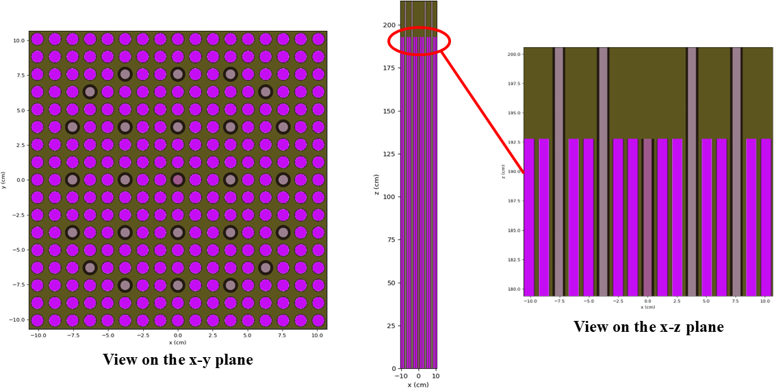
Figure 1: OpenMC geometry colored by material ID shown on the - and - planes
To generate the XML files needed to run OpenMC, you can run the following:
python make_openmc_model.py
Or you can use the model.xml file that is included in the tutorials/lwr_amr directory.
Mesh Generation with the Reactor Module
The mesh used to tally the fission heating in this problem will be generated using the MOOSE Reactor module, which provides a suite of mesh generators suited for common fission reactor geometries. We begin by defining the geometric properties of the assembly (as described in Table 1) followed by some discretization parameters. NUM_SECTORS is the number of azimuthal discretization regions per for a quadrant of the pincell, FUEL_RADIAL_DIVISIONS is the number of radial regions we use for subdividing the fuel, BACKGROUND_DIVISIONS is the number of radial subdivisions for the water bounding box, and AXIAL_DIVISIONS is the number of subdivisions we use when extruding the geometry into 3D.
#----------------------------------------------------------------------------------------
# Assembly geometrical information
#----------------------------------------------------------------------------------------
pitch        = 1.26
fuel_height  = 192.78
r_fuel       = 0.4095
r_fuel_gap   = 0.4180
r_fuel_clad  = 0.4750
r_guide      = 0.3400
r_guide_clad = 0.5400
#----------------------------------------------------------------------------------------

#----------------------------------------------------------------------------------------
# Meshing parameters
#----------------------------------------------------------------------------------------
NUM_SECTORS              = 2
FUEL_RADIAL_DIVISIONS    = 2
BACKGROUND_DIVISIONS     = 1
AXIAL_DIVISIONS          = 5
#----------------------------------------------------------------------------------------After defining the geometric properties and discretization parameters we define the four different pincells in the [Mesh] block using the PolygonConcentricCircleMeshGenerator - the workhorse of the Reactor module. We set preserve_volumes = true in an attempt to preserve the volume of each region, which ensures that our tallied volumetric fission power is consistent with the OpenMC geometry.
  [UO2_Pin]
    type = PolygonConcentricCircleMeshGenerator
    num_sides = 4
    num_sectors_per_side = '${NUM_SECTORS} ${NUM_SECTORS} ${NUM_SECTORS} ${NUM_SECTORS}'
    ring_radii = '${r_fuel} ${r_fuel_gap} ${r_fuel_clad}'
    ring_intervals = '${FUEL_RADIAL_DIVISIONS} 1 1'
    polygon_size = ${fparse pitch / 2.0}

    ring_block_ids = '0 1 2 3'
    ring_block_names = 'uo2_center uo2 fuel_gap zr_clad'
    background_block_ids = '17'
    background_block_names = 'water'
    background_intervals = ${BACKGROUND_DIVISIONS}

    flat_side_up = true
    quad_center_elements = false
    preserve_volumes = true

    create_outward_interface_boundaries = false
  []
  [Control_Rod_Pin]
    type = PolygonConcentricCircleMeshGenerator
    num_sides = 4
    num_sectors_per_side = '${NUM_SECTORS} ${NUM_SECTORS} ${NUM_SECTORS} ${NUM_SECTORS}'
    ring_radii = '${r_guide} ${r_guide_clad}'
    ring_intervals = '${FUEL_RADIAL_DIVISIONS} 1'
    polygon_size = ${fparse pitch / 2.0}

    ring_block_ids = '10 11 12'
    ring_block_names = 'guide_center guide al_clad'
    background_block_ids = '17'
    background_block_names = 'water'
    background_intervals = ${BACKGROUND_DIVISIONS}

    flat_side_up = true
    quad_center_elements = false
    preserve_volumes = true

    create_outward_interface_boundaries = false
  []
  [Fission_Chamber_Pin]
    type = PolygonConcentricCircleMeshGenerator
    num_sides = 4
    num_sectors_per_side = '${NUM_SECTORS} ${NUM_SECTORS} ${NUM_SECTORS} ${NUM_SECTORS}'
    ring_radii = '${r_guide} ${r_guide_clad}'
    ring_intervals = '${FUEL_RADIAL_DIVISIONS} 1'
    polygon_size = ${fparse pitch / 2.0}

    ring_block_ids = '15 16 12'
    ring_block_names = 'fission_center fission al_clad'
    background_block_ids = '17'
    background_block_names = 'water'
    background_intervals = ${BACKGROUND_DIVISIONS}

    flat_side_up = true
    quad_center_elements = false
    preserve_volumes = true

    create_outward_interface_boundaries = false
[]After defining each pincell, these distinct regions are combined into a 2D assembly mesh using a PatternedCartesianMeshGenerator.
  [UO2_Assembly]
    type = PatternedCartesianMeshGenerator
    inputs = 'UO2_Pin Control_Rod_Pin Fission_Chamber_Pin'
    pattern = '0 0 0 0 0 0 0 0 0 0 0 0 0 0 0 0 0;
               0 0 0 0 0 0 0 0 0 0 0 0 0 0 0 0 0;
               0 0 0 0 0 1 0 0 1 0 0 1 0 0 0 0 0;
               0 0 0 1 0 0 0 0 0 0 0 0 0 1 0 0 0;
               0 0 0 0 0 0 0 0 0 0 0 0 0 0 0 0 0;
               0 0 1 0 0 1 0 0 1 0 0 1 0 0 1 0 0;
               0 0 0 0 0 0 0 0 0 0 0 0 0 0 0 0 0;
               0 0 0 0 0 0 0 0 0 0 0 0 0 0 0 0 0;
               0 0 1 0 0 1 0 0 2 0 0 1 0 0 1 0 0;
               0 0 0 0 0 0 0 0 0 0 0 0 0 0 0 0 0;
               0 0 0 0 0 0 0 0 0 0 0 0 0 0 0 0 0;
               0 0 1 0 0 1 0 0 1 0 0 1 0 0 1 0 0;
               0 0 0 0 0 0 0 0 0 0 0 0 0 0 0 0 0;
               0 0 0 1 0 0 0 0 0 0 0 0 0 1 0 0 0;
               0 0 0 0 0 1 0 0 1 0 0 1 0 0 0 0 0;
               0 0 0 0 0 0 0 0 0 0 0 0 0 0 0 0 0;
               0 0 0 0 0 0 0 0 0 0 0 0 0 0 0 0 0'

    pattern_boundary = 'none'

    assign_type = 'cell'
    id_name = 'pin_id'
    generate_core_metadata = false
[]The fuel-cladding gap blocks are deleted after the assembly mesh is generated - this is due to these regions being modelled as voids in OpenMC and so they will not receive any tallies (in other words, we are simply reducing some memory needed to keep unused parts of the mesh, though you could certainly keep those mesh blocks if you desired). We finish the mesh generation process by translating the assembly mesh such that its center is located at the origin, and extrude the geometry from the fuel centerline to the top of the active fuel region.
  [Delete_Blocks]
    type = BlockDeletionGenerator
    input = UO2_Assembly
    # Deleting the gap blocks to avoid erroneous mesh refinement.
    block = '2'
  []
  [To_Origin]
    type = TransformGenerator
    input = 'Delete_Blocks'
    transform = TRANSLATE_CENTER_ORIGIN
  []
  [3D_Core]
    type = AdvancedExtruderGenerator
    input = 'To_Origin'
    heights = '${fparse fuel_height}'
    num_layers = '${AXIAL_DIVISIONS}'
    direction = '0.0 0.0 1.0'
  []
[]
We generate the mesh by running the command below, which creates the mesh_in.e file that is used in the Cardinal input file for volumetric tallies. The final mesh can be found in Figure 2, which is a fairly coarse mesh in the axial direction. We will rely on AMR to refine both the radial and axial power distribution.
cardinal-opt -i mesh.i --mesh-only
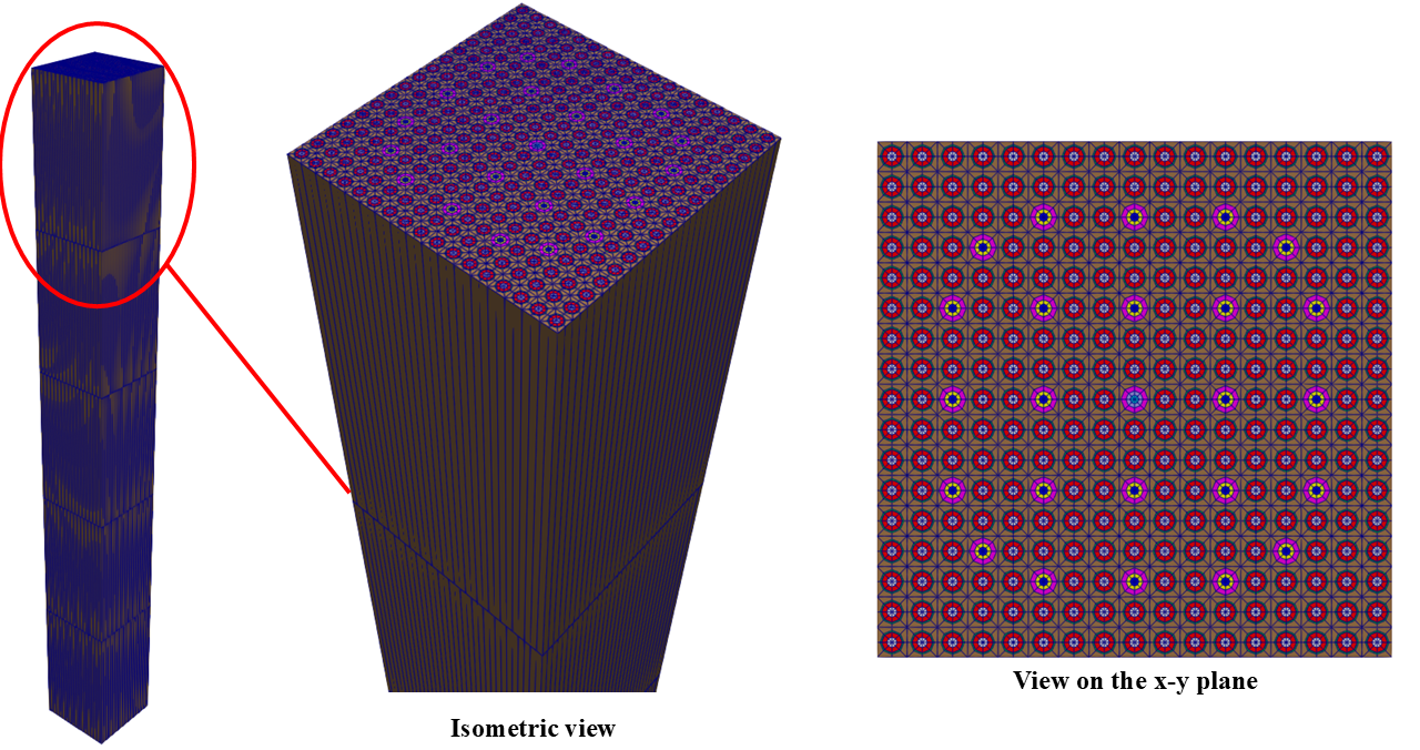
Figure 2: Initial tally mesh colored by block ID, shown in an isometric view and sliced on the plane
Neutronics Input File
The neutronics calculation is performed over the entire assembly by OpenMC, and the wrapping of the OpenMC results in MOOSE is performed in openmc.i. We begin by defining the mesh which will be used by OpenMC to tally the volumetric fission power, which we generated in the previous step:
[Mesh<<<{"href": "../syntax/Mesh/index.html"}>>>]
  [file]
    type = FileMeshGenerator<<<{"description": "Read a mesh from a file.", "href": "../source/meshgenerators/FileMeshGenerator.html"}>>>
    file<<<{"description": "The filename to read."}>>> = mesh_in.e
  []
[]Next, the Problem and Tallies blocks describe all of the syntax necessary to replace the normal MOOSE finite element calculation with an OpenMC neutronics solve. This is done with an OpenMCCellAverageProblem.
[Problem<<<{"href": "../syntax/Problem/index.html"}>>>]
  type = OpenMCCellAverageProblem
  particles = 10000
  inactive_batches = 50
  batches = 1000

  power = '${fparse 3000e6 / 273 * 4}'

  assume_separate_tallies = true
  skip_statepoint = true

  [Tallies<<<{"href": "../syntax/Problem/Tallies/index.html"}>>>]
    [heat_source]
      type = MeshTally<<<{"description": "A class which implements unstructured mesh tallies.", "href": "../source/tallies/MeshTally.html"}>>>
      score<<<{"description": "Score(s) to use in the OpenMC tallies. If not specified, defaults to 'kappa_fission'"}>>> = 'kappa_fission'
      name<<<{"description": "Auxiliary variable name(s) to use for OpenMC tallies. If not specified, defaults to the names of the scores"}>>> = 'heat_source'
      output<<<{"description": "UNRELAXED field(s) to output from OpenMC for each tally score. unrelaxed_tally_std_dev will write the standard deviation of each tally into auxiliary variables named *_std_dev. unrelaxed_tally_rel_error will write the relative standard deviation (unrelaxed_tally_std_dev / unrelaxed_tally) of each tally into auxiliary variables named *_rel_error. unrelaxed_tally will write the raw unrelaxed tally into auxiliary variables named *_raw (replace * with 'name')."}>>> = 'unrelaxed_tally_std_dev'
      block<<<{"description": "Subdomains for which to add tallies in OpenMC. If not provided, tallies will be applied over the entire domain corresponding to the [Mesh] block."}>>> = 'uo2_center uo2'

      normalize_by_global_tally<<<{"description": "Whether to normalize local tallies by a global tally (true) or else by the sum of the local tally (false)"}>>> = false
    []
  []
[]We specify the number of particles to use alongside the assembly power to normalize tally results. We set normalize_by_global_tally = false as the unstructured mesh tally does not perfectly represent the CSG geometry, and so some scores will be missed compared to a global tally. assume_separate_tallies and skip_statepoint are set to true as performance optimizations. A MeshTally is added in the [Tallies] block which will automatically score on mesh_in.e. This tally scores kappa_fission to a MOOSE variable named heat_source while also calculating the standard deviation of the tally field (stored in heat_source_std_dev). We specify that we only wish to tally on the fueled regions (uo2_center and uo2) as the remainder of the assembly will accumulate zero (or near-zero in the case of the fission chamber) tally scores for fission heating.
A steady-state executioner is selected as OpenMC will run a single criticality calculation. We then select exodus and comma-separated values (CSV) output (for our postprocessors) which will occur on the end of the simulation.
[Executioner<<<{"href": "../syntax/Executioner/index.html"}>>>]
  type = Steady
[]

[Outputs<<<{"href": "../syntax/Outputs/index.html"}>>>]
  execute_on<<<{"description": "The list of flag(s) indicating when this object should be executed. For a description of each flag, see https://mooseframework.inl.gov/source/interfaces/SetupInterface.html."}>>> = 'timestep_end'
  exodus<<<{"description": "Output the results using the default settings for Exodus output."}>>> = true
  csv<<<{"description": "Output the scalar variable and postprocessors to a *.csv file using the default CSV output."}>>> = true
[]Finally, we add three TallyRelativeError postprocessors to evaluate the minimum, maximum, and average tally relative error of the kappa_fission score. These are useful for determining if the number of batches need to be increased when increasing the mesh resolution using AMR.
[Postprocessors<<<{"href": "../syntax/Postprocessors/index.html"}>>>]
  [max_rel_err]
    type = TallyRelativeError<<<{"description": "Maximum/minimum tally relative error", "href": "../source/postprocessors/TallyRelativeError.html"}>>>
    value_type<<<{"description": "Whether to give the maximum or minimum tally relative error"}>>> = max
    tally_score<<<{"description": "Score to report the relative error. If there is just a single score, this defaults to that value"}>>> = kappa_fission
  []
  [min_rel_err]
    type = TallyRelativeError<<<{"description": "Maximum/minimum tally relative error", "href": "../source/postprocessors/TallyRelativeError.html"}>>>
    value_type<<<{"description": "Whether to give the maximum or minimum tally relative error"}>>> = min
    tally_score<<<{"description": "Score to report the relative error. If there is just a single score, this defaults to that value"}>>> = kappa_fission
  []
  [avg_rel_err]
    type = TallyRelativeError<<<{"description": "Maximum/minimum tally relative error", "href": "../source/postprocessors/TallyRelativeError.html"}>>>
    value_type<<<{"description": "Whether to give the maximum or minimum tally relative error"}>>> = average
    tally_score<<<{"description": "Score to report the relative error. If there is just a single score, this defaults to that value"}>>> = kappa_fission
  []
[]Execution and Postprocessing
To run the wrapped neutronics calculation,
mpiexec -np 4 cardinal-opt -i openmc.i --n-threads=32
This will run OpenMC with 4 MPI ranks with 32 OpenMP threads per rank. To run the simulation faster, you can increase the parallel processes/threads, or simply decrease the number of particles used in OpenMC. When the simulation has completed, you will have created a number of different output files:
openmc_out.e: an Exodus mesh with the tally results;openmc_out.csv: a CSV file with the results reported by the TallyRelativeError postprocessors.
Figure 3 shows the resulting fission power computed by OpenMC on the mesh tally added by Cardinal. We can see that the radial power distribution peaks near the corners of the assembly (due to the reflective boundary conditions), and is depressed near the guide tubes due to the insertion of the control rods. The center of the assembly sees some additional power peaking due to the fission chamber. The power distribution within the assembly begins to decrease along the z-axis as one moves from the assembly centerline to the vacuum boundary condition. The coarse axial discretization makes it difficult to determine if this follows the standard cosine shape, and the lack of radial refinement fails to capture gradients within each pincell. This motivates the use of AMR to automatically refine the tally mesh.
To add AMR, we add two sub-blocks. The first is the Indicators block, members of which are responsible for computing estimates of the spatial solution error for each element in the mesh. The second is the Markers block, members of which take error estimates from indicators and use them to determine if an element should be isotropically refined or coarsened.
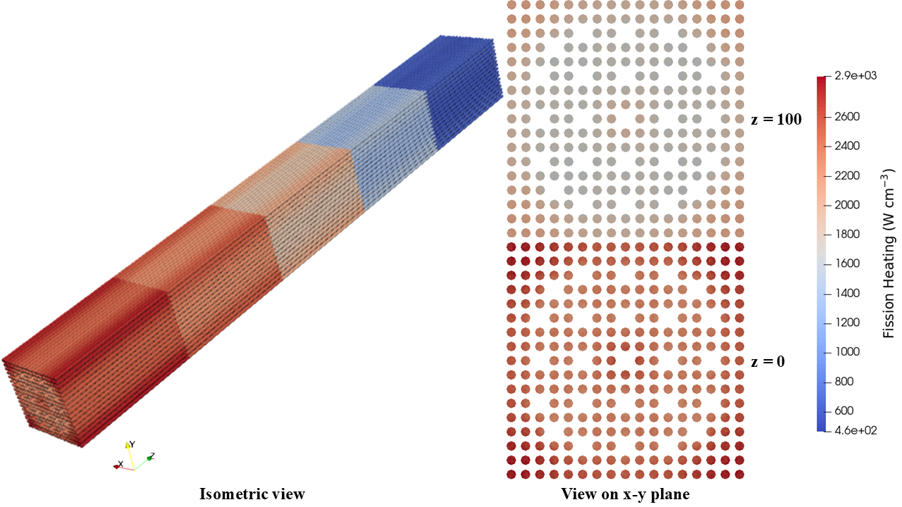
Figure 3: Fission power computed with the unstructured mesh tally, shown with an isometric view and sliced on the plane
Adding Adaptive Mesh Refinement
Next, we will adaptively refine the mesh using the adaptivity system included in MOOSE. The Cardinal input file for adaptivity is largely the same as the input file for the initial mesh tally - it can be found in openmc_amr.i. The main difference between openmc.i and openmc_amr.i is the addition of the Adaptivity block (shown below), which is responsible for determining the refinement / coarsening behaviour of the mesh. The adaptivity block consists of two sub-blocks: Indicators which compute estimates of spatial discretization error, and Markers which use these error estimates to mark elements for refinement or coarsening. Two steps of mesh adaptivity are selected with steps = 2, and error_combo is selected to be the marker to use when modifying the mesh.
[Adaptivity<<<{"href": "../syntax/Adaptivity/index.html"}>>>]
  marker<<<{"description": "The name of the Marker to use to actually adapt the mesh."}>>> = error_combo
  steps<<<{"description": "The number of adaptive steps to use when doing a Steady simulation."}>>> = 2

  [Indicators<<<{"href": "../syntax/Adaptivity/Indicators/index.html"}>>>]
    [optical_depth]
      type = ElementOpticalDepthIndicator<<<{"description": "A class which returns the estimate of a given element's optical depth under the assumption that elements with a large optical depth experience large solution gradients.", "href": "../source/indicators/ElementOpticalDepthIndicator.html"}>>>
      rxn_rate<<<{"description": "The reaction rate to use for computing the optical depth."}>>> = 'fission'
      h_type<<<{"description": "The estimate for the length of the element used to compute the optical depth. Options are the minimum vertex separation (min), the maximum vertex separation (max), and the cube root of the element volume (cube_root)."}>>> = 'max'
    []
  []
  [Markers<<<{"href": "../syntax/Adaptivity/Markers/index.html"}>>>]
    [depth_frac]
      type = ErrorFractionMarker<<<{"description": "Marks elements for refinement or coarsening based on the fraction of the min/max error from the supplied indicator.", "href": "../source/markers/ErrorFractionMarker.html"}>>>
      indicator<<<{"description": "The name of the Indicator that this Marker uses."}>>> = optical_depth
      refine<<<{"description": "Elements within this percentage of the max error will be refined.  Must be between 0 and 1!"}>>> = 0.3
      coarsen<<<{"description": "Elements within this percentage of the min error will be coarsened.  Must be between 0 and 1!"}>>> = 0.0
    []
    [rel_error]
      type = ValueThresholdMarker<<<{"description": "The refinement state based on a threshold value compared to the specified variable.", "href": "../source/markers/ValueThresholdMarker.html"}>>>
      invert<<<{"description": "If this is true then values _below_ 'refine' will be refined and _above_ 'coarsen' will be coarsened."}>>> = true
      coarsen<<<{"description": "The threshold value for coarsening.  Elements with variable values beyond this will be marked for coarsening."}>>> = 1e-1
      refine<<<{"description": "The threshold value for refinement.  Elements with variable values beyond this will be marked for refinement."}>>> = 5e-2
      variable<<<{"description": "The values of this variable will be compared to 'refine' and 'coarsen' to see what should be done with the element"}>>> = heat_source_rel_error
      third_state<<<{"description": "The Marker state to apply to values falling in-between the coarsen and refine thresholds."}>>> = DO_NOTHING
    []
    [error_combo]
      type = BooleanComboMarker<<<{"description": "A class which takes multiple markers and ANDs / ORs them together to determine if an element should be refined or coarsened.", "href": "../source/markers/BooleanComboMarker.html"}>>>
      # Only refine iff the relative error is sufficiently low AND the optical depth is
      # sufficiently large.
      refine_markers<<<{"description": "A list of the marker names to be used for refinement."}>>> = 'rel_error depth_frac'
      # Coarsen based exclusively on relative error.
      coarsen_markers<<<{"description": "A list of the marker names to be used for coasening."}>>> = 'rel_error'
      boolean_operator<<<{"description": "How the different markers should be combined. Options are to AND each marker together or to OR them together."}>>> = and
    []
  []
[]In this adaptivity block we define a single indicator which assumes that the spatial error in an element is proportional to the mean optical depth within the element (optical_depth). This indicator requires a tally score to use for computing the energy-integrated reaction rate in an element - we select the fission reaction rate as we aim to optimize the spatial distribution of fission heating. It also requires an estimate of the mean chord length in the element (h_type) which we set to the maximum vertex separation in an element due to the coarse axial discretization in our initial mesh.
We then add three markers, the first of which is a ErrorFractionMarker (depth_frac) which takes optical_depth as an input. This marker sorts all elements into descending order based on the indicator value, then iterates over the list (starting with the largest error estimate). Elements whose optical depth sum to a refinement fraction multiplied by the total error estimate are refined. The list is iterated in reverse to mark elements for coarsening. We set the refinement fraction refine = 0.3, while setting the coarsening threshold coarsen = 0.0. The next marker we add is a ValueThresholdMarker (rel_error), which marks elements for refinement if their value is above refine and marks elements to be coarsened if their value is above coarsen. We pass it the variable containing the relative error of the fission heating (variable = heat_source_rel_error) and set invert = true. This has the effect of marking an element for coarsening if the fission heating relative error is above 1e-1, while allowing refinement of the relative error of the fission heating relative error is below 5e-2. We set third_state = DO_NOTHING to indicate that elements in this region should not be refined or coarsened. The final marker we add is a BooleanComboMarker (error_combo) which combines the previous two markers based on a flag in boolean_operator. refine_markers = 'rel_error depth_frac' with the and boolean flag results in refinement only when the element is marked based on it's fraction of the optical depth and has a sufficiently low statistical relative error. coarsen_markers = 'rel_error' results in coarsening only if the element has a sufficiently hight statistical relative error.
The remaining modifications that need to be made are done to support [Adaptivity]. We modify heat_source to also score flux and fission to allow for the calculation of the optical depth. This also necessitates the specification of source_rate_normalization = 'kappa_fission' as two non-heating scores have been added. unrelaxed_tally_rel_error is added to the output parameter to enable the rel_error marker. The modifications to the [Problem] and [Tallies] block can be found below.
[Problem<<<{"href": "../syntax/Problem/index.html"}>>>]
  type = OpenMCCellAverageProblem
  particles = 10000
  inactive_batches = 50
  batches = 1000

  power = '${fparse 3000e6 / 273 * 4}'
  source_rate_normalization = 'kappa_fission'

  assume_separate_tallies = true
  skip_statepoint = true

  [Tallies<<<{"href": "../syntax/Problem/Tallies/index.html"}>>>]
    [heat_source]
      type = MeshTally<<<{"description": "A class which implements unstructured mesh tallies.", "href": "../source/tallies/MeshTally.html"}>>>
      score<<<{"description": "Score(s) to use in the OpenMC tallies. If not specified, defaults to 'kappa_fission'"}>>> = 'kappa_fission fission flux'
      name<<<{"description": "Auxiliary variable name(s) to use for OpenMC tallies. If not specified, defaults to the names of the scores"}>>> = 'heat_source fission flux'
      output<<<{"description": "UNRELAXED field(s) to output from OpenMC for each tally score. unrelaxed_tally_std_dev will write the standard deviation of each tally into auxiliary variables named *_std_dev. unrelaxed_tally_rel_error will write the relative standard deviation (unrelaxed_tally_std_dev / unrelaxed_tally) of each tally into auxiliary variables named *_rel_error. unrelaxed_tally will write the raw unrelaxed tally into auxiliary variables named *_raw (replace * with 'name')."}>>> = 'unrelaxed_tally_std_dev unrelaxed_tally_rel_error'
      block<<<{"description": "Subdomains for which to add tallies in OpenMC. If not provided, tallies will be applied over the entire domain corresponding to the [Mesh] block."}>>> = 'uo2_center uo2'

      normalize_by_global_tally<<<{"description": "Whether to normalize local tallies by a global tally (true) or else by the sum of the local tally (false)"}>>> = false
    []
  []
[]The final change we make is to add an extra postprocessor named num_elem to output the number of elements. This postprocessor filters for the number of active elements, which are the elements currently being tallied on. This is distinct from the total number of elements as MOOSE/libMesh maintains the entire refinement hierarchy, and so elements which aren't participating in the solve at the current refinement cycle still exist in memory (and therefore are included in the total element count).
[Postprocessors<<<{"href": "../syntax/Postprocessors/index.html"}>>>]
  [num_elem]
    type = NumElements<<<{"description": "Return the number of active or total elements in the simulation.", "href": "../source/postprocessors/NumElements.html"}>>>
    elem_filter<<<{"description": "The type of elements to include in the count (active, total). Default == active"}>>> = active
  []
  [max_rel_err]
    type = TallyRelativeError<<<{"description": "Maximum/minimum tally relative error", "href": "../source/postprocessors/TallyRelativeError.html"}>>>
    value_type<<<{"description": "Whether to give the maximum or minimum tally relative error"}>>> = max
    tally_score<<<{"description": "Score to report the relative error. If there is just a single score, this defaults to that value"}>>> = kappa_fission
  []
  [min_rel_err]
    type = TallyRelativeError<<<{"description": "Maximum/minimum tally relative error", "href": "../source/postprocessors/TallyRelativeError.html"}>>>
    value_type<<<{"description": "Whether to give the maximum or minimum tally relative error"}>>> = min
    tally_score<<<{"description": "Score to report the relative error. If there is just a single score, this defaults to that value"}>>> = kappa_fission
  []
  [avg_rel_err]
    type = TallyRelativeError<<<{"description": "Maximum/minimum tally relative error", "href": "../source/postprocessors/TallyRelativeError.html"}>>>
    value_type<<<{"description": "Whether to give the maximum or minimum tally relative error"}>>> = average
    tally_score<<<{"description": "Score to report the relative error. If there is just a single score, this defaults to that value"}>>> = kappa_fission
  []
[]Execution and Postprocessing
To run the neutronics calculation with AMR,
mpiexec -np 4 cardinal-opt -i openmc_amr.i --n-threads=32
First, lets examine how the reported relative errors and the number of elements in the problem changes as the mesh is adaptively refined / coarsened:
Postprocessor Values:
+----------------+----------------+----------------+----------------+----------------+
| time           | avg_rel_err    | max_rel_err    | min_rel_err    | num_elem       |
+----------------+----------------+----------------+----------------+----------------+
|   1.000000e+00 |   1.721342e-02 |   3.750385e-02 |   8.727138e-03 |   4.624000e+04 |
|   2.000000e+00 |   4.803123e-02 |   1.500115e-01 |   2.182817e-02 |   1.940800e+05 |
|   3.000000e+00 |   6.194000e-02 |   1.979877e-01 |   2.188693e-02 |   2.466990e+05 |
+----------------+----------------+----------------+----------------+----------------+
We can see that avg_rel_err starts at ~1% on the first iteration and jumps to ~4% on the second iteration, which is corroborated by num_elem quadrupling on this step (from 46240 to 194080) indicating that a large amount of refinement is taking place. This behavior slows down on the third step as the number of elements remaining that meet both the spatial refinement criteria (optical depth) and the statistical error requirement (relative error less than 5%) are limited, and so the average relative error only increases to ~6% while another 52619 elements are added. Looking at max_rel_err we can also see that some elements meet the statistical error criteria before refinement, but after refinement their relative error overshoots the maximum error threshold and so the maximum relative error in the problem jumps to ~20%. We can see this behavior in Figure 4 where the heat source is initially refined semi-uniformly over the domain. Then, the elements near the core centerline and the edges of the assembly are marked for refinement due to an increase in the estimated optical depth from higher fission rates. After the third iteration the edge of the assembly nearest to the vacuum boundary and the corners of the assembly are marked for coarsening due to the jump in relative error. Running the simulation with additional particles per batch or more active batches would further decrease the per-element relative error and allow for added refinement steps. The jumps in relative error above the upper limit of 10% can also be mitigated by decreasing the refinement threshold in rel_error from 5% to 1%.
 assembly over multiple adaptivity cycles.](../media/assembly_amr_res.gif)
Figure 4: Elements marked for refinement (left), fission power (middle), and elements marked for coarsening (right) for the LWR assembly over multiple adaptivity cycles.
Single Pincell
In this section, we isolate a single pin from the corner of the assembly mesh to tally and run adaptivity on. The mesh input file (mesh_pin.i) can be found below. We first generate a UO pin, and translate it to ensure it lines up with a fuel pin (as the central pin in the assembly is a fission chamber). This pin is then extruded to the full length of the fueled region and the gap block is deleted (as it will never be tallied on).
#----------------------------------------------------------------------------------------
# Assembly geometrical information
#----------------------------------------------------------------------------------------
pitch        = 1.26
fuel_height  = 192.78
r_fuel       = 0.4095
r_fuel_gap   = 0.4180
r_fuel_clad  = 0.4750
r_guide      = 0.3400
r_guide_clad = 0.5400
#----------------------------------------------------------------------------------------

#----------------------------------------------------------------------------------------
# Meshing parameters
#----------------------------------------------------------------------------------------
NUM_SECTORS              = 2
FUEL_RADIAL_DIVISIONS    = 2
BACKGROUND_DIVISIONS     = 1
AXIAL_DIVISIONS          = 5
#----------------------------------------------------------------------------------------

[Mesh<<<{"href": "../syntax/Mesh/index.html"}>>>]
  [UO2_Pin]
    type = PolygonConcentricCircleMeshGenerator<<<{"description": "This PolygonConcentricCircleMeshGenerator object is designed to mesh a polygon geometry with optional rings centered inside.", "href": "../source/meshgenerators/PolygonConcentricCircleMeshGenerator.html"}>>>
    num_sides<<<{"description": "Number of sides of the polygon."}>>> = 4
    num_sectors_per_side<<<{"description": "Number of azimuthal sectors per polygon side (rotating counterclockwise from top right face)."}>>> = '${NUM_SECTORS} ${NUM_SECTORS} ${NUM_SECTORS} ${NUM_SECTORS}'
    ring_radii<<<{"description": "Radii of major concentric circles (rings)."}>>> = '${r_fuel} ${r_fuel_gap} ${r_fuel_clad}'
    ring_intervals<<<{"description": "Number of radial mesh intervals within each major concentric circle excluding their boundary layers."}>>> = '${FUEL_RADIAL_DIVISIONS} 1 1'
    polygon_size<<<{"description": "Size of the polygon to be generated (given as either apothem or radius depending on polygon_size_style)."}>>> = ${fparse pitch / 2.0}

    ring_block_ids<<<{"description": "Optional customized block ids for each ring geometry block."}>>> = '0 1 2 3'
    ring_block_names<<<{"description": "Optional customized block names for each ring geometry block."}>>> = 'uo2_center uo2 fuel_gap zr_clad'
    background_block_ids<<<{"description": "Optional customized block id for the background block."}>>> = '17'
    background_block_names<<<{"description": "Optional customized block names for the background block."}>>> = 'water'
    background_intervals<<<{"description": "Number of radial meshing intervals in background region (area between rings and ducts) excluding the background's boundary layers."}>>> = ${BACKGROUND_DIVISIONS}

    flat_side_up<<<{"description": "Whether to rotate the generated polygon mesh to ensure that one flat side faces up."}>>> = true
    quad_center_elements<<<{"description": "Whether the center elements are quad or triangular."}>>> = false
    preserve_volumes<<<{"description": "Volume of concentric circles can be preserved using this function."}>>> = true

    create_outward_interface_boundaries<<<{"description": "Whether the outward interface boundaries are created."}>>> = false
  []
  [Delete_Blocks]
    type = BlockDeletionGenerator<<<{"description": "Mesh generator which removes elements from the specified subdomains", "href": "../source/meshgenerators/BlockDeletionGenerator.html"}>>>
    input<<<{"description": "The mesh we want to modify"}>>> = UO2_Pin
    # Deleting the gap blocks to avoid erroneous mesh refinement.
    block<<<{"description": "The list of blocks to be processed (deleted or kept)"}>>> = '2'
  []
  [Left]
    type = TransformGenerator<<<{"description": "Applies a linear transform to the entire mesh.", "href": "../source/meshgenerators/TransformGenerator.html"}>>>
    input<<<{"description": "The mesh we want to modify"}>>> = 'Delete_Blocks'
    transform<<<{"description": "The type of transformation to perform (TRANSLATE, TRANSLATE_CENTER_ORIGIN, TRANSLATE_MIN_ORIGIN, ROTATE, SCALE, ROTATE_WITH_MATRIX, ROTATE_EXT)"}>>> = TRANSLATE
    vector_value<<<{"description": "The value to use for the transformation. When using TRANSLATE or SCALE, the xyz coordinates are applied in each direction respectively. When using ROTATE, the values are interpreted as the Euler angles phi, theta and psi given in degrees. For ROTATE_EXT, an extrinsic rotation is carried out using prescribed Euler angles alpha, beta, and gamma in degrees."}>>> = '${fparse -1 * pitch} ${fparse -1 * pitch} 0.0'
  []
  [3D_Core]
    type = AdvancedExtruderGenerator<<<{"description": "Extrudes a 1D mesh into 2D, or a 2D mesh into 3D, and supports a variable height for each elevation, variable number of layers within each elevation, variable growth factors of axial element sizes within each elevation and remap subdomain_ids, boundary_ids and element extra integers within each elevation as well as interface boundaries between neighboring elevation layers, as well as following a 1D curve and modifying the radial (normal to the extrusion axis) extent of the geometry.", "href": "../source/meshgenerators/AdvancedExtruderGenerator.html"}>>>
    input<<<{"description": "The mesh to extrude"}>>> = 'Left'
    heights<<<{"description": "The height of each elevation"}>>> = '${fparse fuel_height}'
    num_layers<<<{"description": "The number of layers for each elevation - must be num_elevations in length!"}>>> = '${AXIAL_DIVISIONS}'
    direction<<<{"description": "A vector that points in the direction to extrude (note, this will be normalized internally - so don't worry about it here)"}>>> = '0.0 0.0 1.0'
  []
[]The mesh can be generated by running:
cardinal-opt -i mesh_pin.i --mesh-only
The first modification made to openmc_amr.i is to change the mesh block such that it tallies on the single pin mesh:
[Mesh<<<{"href": "../syntax/Mesh/index.html"}>>>]
  [file]
    type = FileMeshGenerator<<<{"description": "Read a mesh from a file.", "href": "../source/meshgenerators/FileMeshGenerator.html"}>>>
    file<<<{"description": "The filename to read."}>>> = mesh_pin_in.e
  []
[]The second modification is to set particles = 1000 to ensure this problem is runnable with modest computational resources:
[Problem<<<{"href": "../syntax/Problem/index.html"}>>>]
  type = OpenMCCellAverageProblem
  particles = 1000
  inactive_batches = 50
  batches = 1000

  power = '${fparse 3000e6 / 273 * 4}'
  source_rate_normalization = 'kappa_fission'

  assume_separate_tallies = true
  skip_statepoint = true

  [Tallies<<<{"href": "../syntax/Problem/Tallies/index.html"}>>>]
    [heat_source]
      type = MeshTally<<<{"description": "A class which implements unstructured mesh tallies.", "href": "../source/tallies/MeshTally.html"}>>>
      score<<<{"description": "Score(s) to use in the OpenMC tallies. If not specified, defaults to 'kappa_fission'"}>>> = 'kappa_fission fission flux'
      name<<<{"description": "Auxiliary variable name(s) to use for OpenMC tallies. If not specified, defaults to the names of the scores"}>>> = 'heat_source fission flux'
      output<<<{"description": "UNRELAXED field(s) to output from OpenMC for each tally score. unrelaxed_tally_std_dev will write the standard deviation of each tally into auxiliary variables named *_std_dev. unrelaxed_tally_rel_error will write the relative standard deviation (unrelaxed_tally_std_dev / unrelaxed_tally) of each tally into auxiliary variables named *_rel_error. unrelaxed_tally will write the raw unrelaxed tally into auxiliary variables named *_raw (replace * with 'name')."}>>> = 'unrelaxed_tally_std_dev unrelaxed_tally_rel_error'
      block<<<{"description": "Subdomains for which to add tallies in OpenMC. If not provided, tallies will be applied over the entire domain corresponding to the [Mesh] block."}>>> = 'uo2_center uo2'

      normalize_by_global_tally<<<{"description": "Whether to normalize local tallies by a global tally (true) or else by the sum of the local tally (false)"}>>> = false
    []
  []
[]Execution and Postprocessing
To run the single pin problem,
mpiexec -np 2 cardinal-opt -i openmc_amr_single.i --n-threads=2
First, lets examine how the reported relative errors and the number of elements in the problem changes as the mesh is adaptively refined / coarsened:
Postprocessor Values:
+----------------+----------------+----------------+----------------+----------------+
| time           | avg_rel_err    | max_rel_err    | min_rel_err    | num_elem       |
+----------------+----------------+----------------+----------------+----------------+
|   1.000000e+00 |   5.435691e-02 |   1.121199e-01 |   2.985789e-02 |   1.600000e+02 |
|   2.000000e+00 |   9.696449e-02 |   1.707078e-01 |   4.991084e-02 |   4.120000e+02 |
|   3.000000e+00 |   9.169795e-02 |   1.555218e-01 |   4.561517e-02 |   3.770000e+02 |
+----------------+----------------+----------------+----------------+----------------+
The behavior of the relative error for the single pincell is similar to the full assembly case, though the reduced number of particles per batch decreases the amount of refinement that the model can support. avg_rel_err starts at ~5% on the first iteration, and then jumps to ~9% due to the addition of more elements on the second iteration. The selected adaptivity scheme then coarsens those elements which results in a decrease in max_rel_err from ~17% on iteration two to ~15% on iteration three - the maximum doesn't decrease a substantial amount as certain elements have a relative error less than 5% and refine to a relative error larger than 10%. We can see this behaviourin Figure 5, where the adaptivity algorithm initially over-refines and then coarsens to ensure the relative error of the tally bins is between 5% and 10%
Figure 5: Elements marked for refinement (left), fission power (middle), and elements marked for coarsening (right) for a single pincell over multiple adaptivity cycles.
References
- S. Cathalau, J. C. Lefebvre, and J. P. West.
Proposal for a Second Stage of the Benchmark on Power Distributions within Assemblies.
Technical Report NEA/NSC/DOC(96)2, Organisation for Economic Cooperation and Development, Nuclear Energy Agency, 1996.
URL: https://www.oecd-nea.org/upload/docs/application/pdf/2020-01/nsc-doc96-02-rev2.pdf.[Export]
- M.A. Smith, E.E. Lewis, and Byung-Chan Na.
Benchmark on Deterministic 3-D MOX Fuel Assembly Transport Calculations without Spatial Homogenization.
Progress in Nuclear Energy, 48(5):383–393, 2006.
doi:https://doi.org/10.1016/j.pnucene.2006.01.002.[Export]