Conjugate Heat Transfer for Reflector Bypass Flow

In this tutorial, you will learn how to:

Couple NekRS with MOOSE for CHT in a pebble bed reactor reflector block
Propagate scalar values into the OCCA GPU kernels

To access this tutorial,


cd cardinal/tutorials/fhr_reflector

This tutorial also requires you to download some mesh files and restart files from Box. Please download the files from the fhr_reflector folder here and place these files within the same directory structure in tutorials/fhr_reflector.

This tutorial was developed with funding from the NRIC Virtual Test Bed (VTB). You can find additional context on this model in our conference publication Novak et al. (2021).

note:Computing Needs

This tutorial requires HPC resources to run.

Geometry and Computational Model

The pebble region in the Pebble Bed Fluoride-Salt-Cooled High-Temperature Reactor (PB-FHR) is enclosed by an outer graphite reflector. In order to keep the graphite reflector within allowable design temperatures, the reflector contains several bypass flow paths so that a small percentage of the coolant flow can maintain the graphite within allowable temperature ranges. This bypass flow is important to quantify so that accurate estimates of core cooling and reflector temperatures can be obtained. By repeating these calculations for a range of Reynolds numbers and geometries, this model can be used to provide friction factor and Nusselt number correlations.

This section describes the PB-FHR reflector geometry and our computational model. A top-down view of the PB-FHR reactor is shown in Figure 1, with important specifications summarized in Table 1. The center region is the pebble bed core, which is surrounded by two rings of graphite reflector blocks, staggered in a brick-like fashion. The nominal gap size between blocks is 0.002 m, but to ease meshing and make model depiction easier, the gap between blocks is increased to 0.006 m (which could be interpreted as an end-of-life, maximum-swelling condition Novak et al. (2021)). Each ring contains 24 blocks. In black is shown the core barrel. To form the entire axial height of the reflector, rings of blocks are stacked vertically. The entire core height is 5.3175 m, or about 10 vertical rings of blocks. Additional structures are present as well, but are not considered here.

Top-down schematic of the [!ac](PB-FHR) reactor core.

Figure 1: Top-down schematic of the PB-FHR reactor core.

Table 1: Geometric and operating conditions relevant to reflector block modeling, based on Shaver et al. (2019)

Parameter	Value
Pebble core radius	2.6 m
Inner block radial thickness	0.3 m
Outer block radial thickness	0.4 m
Barrel thickness	0.022 m
Gap between blocks	0.006 m
Gap between blocks and barrel	0.02 m
Block height	0.52 m
Core inlet temperature	600°C
Core outlet temperature	700°C

FLiBe flows through the pebble bed, through small gaps between reflector blocks, and between small gaps between the reflector blocks and the barrel. These bypass paths are shown as yellow dashed lines in Figure 1. Due to the top-down orientation of Figure 1, flow paths radially (i.e. from lower to higher $var element = document.getElementById("moose-equation-e7b836c4-f763-4845-a572-7e6aba73039e");katex.render("r", element, {displayMode:false,throwOnError:false});$ at a fixed $var element = document.getElementById("moose-equation-05cebfe7-1a43-40fa-b9fe-b9a4c55c9206");katex.render("z", element, {displayMode:false,throwOnError:false});$ between stacks of reflector blocks) are not shown. While such radial bypass paths contribute to bypass flow, they are not considered here.

The coupled NekRS-MOOSE simulation is conducted for a single ring of reflector blocks (i.e. a height of 0.52 m), with azimuthal symmetry assumed to further reduce the domain to half of an inner ring block, half of an outer ring block, and the vertical bypass flow paths between the blocks and the barrel. This computational domain is shown outlined with a red dotted line in Figure 1.

Heat Conduction Model

The MOOSE heat transfer module is used to solve for energy conservation in the solid. A fixed heat flux of 5 kW/m $var element = document.getElementById("moose-equation-518c5c95-87ea-4c58-a3ce-7c20c2b68541");katex.render("^2", element, {displayMode:false,throwOnError:false});$ is imposed on the block surface facing the pebble bed. On the surface of the barrel, a heat convection boundary condition is imposed,

$(1)var element = document.getElementById("moose-equation-ada5f7a6-a97f-47ef-bfbf-9815d1e926c6");katex.render(" q^{''}=h\\left(T_s-T_\\infty\\right)", element, {displayMode:true,throwOnError:false});$

where $var element = document.getElementById("moose-equation-44b431f5-ecb2-4c84-960b-37080aa7fb2a");katex.render("q^{''}", element, {displayMode:false,throwOnError:false});$ is the heat flux, $var element = document.getElementById("moose-equation-28914d65-4fef-4d1b-8833-de1d7e9a3f3c");katex.render("h", element, {displayMode:false,throwOnError:false});$ is the convective heat transfer coefficient, and $var element = document.getElementById("moose-equation-a9988aab-d6c3-41fe-b6e3-69510b14df7d");katex.render("T_\\infty", element, {displayMode:false,throwOnError:false});$ is the far-field ambient temperature. At fluid-solid interfaces, the solid temperature is imposed as a Dirichlet condition, where NekRS computes the surface temperature. All other solid boundaries are treated as insulated.

NekRS Model

NekRS is used to solve the incompressible Navier-Stokes equations in non-dimensional form. In this tutorial, the following characteristic scales are selected:

$var element = document.getElementById("moose-equation-310c9ada-845e-4431-ad76-b731aed556ca");katex.render("L_{ref}=0.006", element, {displayMode:false,throwOnError:false});$ m, such that the block gap width is unity
$var element = document.getElementById("moose-equation-bf09a2d6-3c89-4f81-94cb-75ab5e6c302d");katex.render("u_{ref}=0.0575", element, {displayMode:false,throwOnError:false});$ m/s, which corresponds to a Reynolds number of 100
$var element = document.getElementById("moose-equation-0703cbaa-d9d7-4dda-9f4e-c598a6123765");katex.render("T_{ref} = 923.15", element, {displayMode:false,throwOnError:false});$ K, the inlet temperature
$var element = document.getElementById("moose-equation-84e8be9c-f8b9-43c6-b1b9-95b16b90c408");katex.render("\\Delta T=10", element, {displayMode:false,throwOnError:false});$ K, an arbitrary selection

A Reynolds number of 100 corresponds to a bypass fraction of about 7%, considering that $var element = document.getElementById("moose-equation-e142389f-15df-437f-bef7-7a4453a88b57");katex.render("Re", element, {displayMode:false,throwOnError:false});$ can be written equivalently as

$(2)var element = document.getElementById("moose-equation-040bba42-67fb-4f12-912b-8a6672181c9c");katex.render(" Re\\equiv\\frac{\\dot{m}L_{ref}}{A\\mu}", element, {displayMode:true,throwOnError:false});$

where $var element = document.getElementById("moose-equation-6ff268e2-4188-49e6-a116-978be03b7091");katex.render("\\dot{m}", element, {displayMode:false,throwOnError:false});$ is the mass flowrate (a fraction of the total core mass flowrate, distributed among 48 half-reflector blocks) and $var element = document.getElementById("moose-equation-ceedbb1b-35d6-4d90-8ef2-a84033ecc970");katex.render("A", element, {displayMode:false,throwOnError:false});$ is the inlet flow area.

The only characteristic scale that requires additional comment is $var element = document.getElementById("moose-equation-d62f901b-e71a-468a-bfd3-bbe13d6ff401");katex.render("\\Delta T", element, {displayMode:false,throwOnError:false});$ - this parameter truly is arbitrary, since it does not appear in the definitions of $var element = document.getElementById("moose-equation-04b05516-efcb-4825-955f-f1b5804a48ba");katex.render("Re", element, {displayMode:false,throwOnError:false});$ or $var element = document.getElementById("moose-equation-ed5b5f94-b5ee-4882-bcab-46ad118dc32b");katex.render("Pe", element, {displayMode:false,throwOnError:false});$ (and, none of the initial conditions/kernels in NekRS's case files assume any range for temperature). That is, if the converged solution has an inlet temperature of 400 K and an outlet temperature of 500 K, setting $var element = document.getElementById("moose-equation-04b69a99-9cf8-49b8-848d-d688d5f851df");katex.render("\\Delta T=100", element, {displayMode:false,throwOnError:false});$ means that $var element = document.getElementById("moose-equation-3391f5ba-1803-4278-9eac-0012a1792a8d");katex.render("T^\\dagger", element, {displayMode:false,throwOnError:false});$ will range from 0 to 1. Setting a different value, such as $var element = document.getElementById("moose-equation-0a3a4a01-8101-4470-84a7-5dc9e744d3b1");katex.render("\\Delta T=50", element, {displayMode:false,throwOnError:false});$ , means that $var element = document.getElementById("moose-equation-097b1fec-d536-4a71-b46c-f470de9ad037");katex.render("T^\\dagger", element, {displayMode:false,throwOnError:false});$ will instead range from 0 to 2. The only scenario where $var element = document.getElementById("moose-equation-30a56648-d6a7-431d-b766-ae263f88c9b9");katex.render("\\Delta T", element, {displayMode:false,throwOnError:false});$ is of consequences is if you are setting initial conditions for temperature or have imposed a heat source yourself within the .oudf file.

At the inlet, the fluid temperature is taken as 650°C, or the nominal median fluid temperature. The inlet velocity is set to a uniform value such that the Reynolds number is 100. At the outlet, a zero pressure is imposed. On the $var element = document.getElementById("moose-equation-a9afafc1-2950-40eb-9f0c-7652b767ba16");katex.render("\\theta=0^\\circ", element, {displayMode:false,throwOnError:false});$ boundary (i.e. the $var element = document.getElementById("moose-equation-22626802-db73-43bb-8d83-3d61682c0f83");katex.render("y=0", element, {displayMode:false,throwOnError:false});$ boundary), symmetry is imposed such that all derivatives in the $var element = document.getElementById("moose-equation-8d1ba3dc-fb06-4a3a-950e-0bdf3c867a17");katex.render("y", element, {displayMode:false,throwOnError:false});$ direction are zero. All other boundaries are treated as no-slip.

note

The $var element = document.getElementById("moose-equation-8c1c7fae-5694-4dab-8506-23f4fd0c31d9");katex.render("\\theta=7.5^\\circ", element, {displayMode:false,throwOnError:false});$ boundary (i.e. $var element = document.getElementById("moose-equation-77d750c8-7b15-4a7d-8fa5-88598e1e4c39");katex.render("360^\\circ", element, {displayMode:false,throwOnError:false});$ divided by 24 blocks, divided in half because we are modeling only half a block) should also be imposed as a symmetry boundary in the NekRS model. However, at the time when we first made this tutorial, NekRS only supported symmetry boundaries for sidesets aligned with the $var element = document.getElementById("moose-equation-c6167c94-5b46-4f2d-8590-0a30ece857f8");katex.render("x", element, {displayMode:false,throwOnError:false});$ , $var element = document.getElementById("moose-equation-3c72bde4-4aed-4d4f-8ade-e800c454ab9e");katex.render("y", element, {displayMode:false,throwOnError:false});$ , and $var element = document.getElementById("moose-equation-9e651f03-7880-42b9-a31e-5fcb3a3d8fe6");katex.render("z", element, {displayMode:false,throwOnError:false});$ coordinate axes. Here, a no-slip boundary condition is used instead, so the correspondence of the NekRS computational model to the depiction in Geometry and Computational Model is imperfect. This is no longer a restriction in NekRS.

At fluid-solid interfaces, the heat flux is imposed as a Neumann condition, where MOOSE computes the surface heat flux.

Because the NekRS mesh contains very small elements in the fluid phase, fairly small time steps are required to meet CFL conditions related to stability. Therefore, the approach to the coupled, pseudo-steady CHT solution can be accelerated by obtaining initial conditions from a pure conduction simulation. Then, the initial conditions for the CHT simulation will begin from the temperature obtained from the conduction simulation, with a uniform axial velocity and zero pressure. The process to run Cardinal in conduction mode is described in Part 1: Initial Conduction Coupling , while the process to run Cardinal in CHT mode is described in Part 2: CHT Coupling .

Meshing

Cubit SNL (2012) is used to programmatically create meshes with user-defined geometry and customizable boundary layers. Journal files, or Python-scripted Cubit inputs, are used to create meshes in Exodus II format. The MOOSE framework accepts meshes in a wide range of formats that can be generated with many commercial and free meshing tools; other tutorials will make meshes natively within MOOSE.

Solid Mesh

The Cubit script used to generate the solid mesh is shown below. To run this script yourself, open Cubit and click on 'Play Journal File' (the play button on a sheet of paper icon), and then find and open your file. Also, you will need to update the directory variable to point to the tutorials directory on your machine.

#!python

# This is a mesh of half of 1/24th of the outer reflector ring in a pebble bed
# fluoride-salt-cooled high temperature reactor (there are 24
# blocks per ring), in addition to the barrel. Only the solid phase is modeled.

import math

# multiplicative factor to apply to the gap width; the nominal gap width cited
# in Shaver et. al (2019) corresponds to a gap amplification factor of 1.0.
gap_amplification = 3

# Path to the tutorials directory on your computer, if you want to run this script
# this will need to be updated
directory = '/Users/anovak/projects/cardinal/tutorials/'

core_radius       = 2.6
layer1_thickness  = 0.3
layer2_thickness  = 0.4
block_gap         = 0.002 * gap_amplification
bypass_gap        = 0.02
height            = 0.502
barrel_thickness  = 0.022
n_blocks_per_ring = 24
angle             = 360 / n_blocks_per_ring

barrel_outer_radius = core_radius + layer1_thickness + block_gap + layer2_thickness +\
                      bypass_gap + barrel_thickness

barrel_inner_radius = barrel_outer_radius - barrel_thickness

layer2_outer_radius = barrel_inner_radius - bypass_gap

layer2_inner_radius = layer2_outer_radius - layer2_thickness

layer1_outer_radius = layer2_inner_radius - block_gap

layer1_inner_radius = layer1_outer_radius - layer1_thickness

cubit.cmd('create cylinder radius ' + str(barrel_outer_radius) + ' height ' + str(height))
cubit.cmd('create cylinder radius ' + str(barrel_inner_radius) + ' height ' + str(height))
cubit.cmd('subtract volume 2 from volume 1')
cubit.cmd('compress all')
cubit.cmd('merge all')

cubit.cmd('create cylinder radius ' + str(layer2_outer_radius) + ' height ' + str(height))
cubit.cmd('create cylinder radius ' + str(layer2_inner_radius) + ' height ' + str(height))
cubit.cmd('subtract volume 3 from volume 2')
cubit.cmd('compress all')
cubit.cmd('merge all')

cubit.cmd('create cylinder radius ' + str(layer1_outer_radius) + ' height ' + str(height))
cubit.cmd('create cylinder radius ' + str(layer1_inner_radius) + ' height ' + str(height))
cubit.cmd('subtract volume 4 from volume 3')
cubit.cmd('compress all')
cubit.cmd('merge all')

l = block_gap / 2.0
cubit.cmd('create brick x ' + str(2.0 * barrel_outer_radius) + ' y ' + str(2.0 * barrel_outer_radius) + ' z ' + str(height))
cubit.cmd('move volume 4 y ' + str(-barrel_outer_radius - l))
cubit.cmd('subtract volume 4 from volume 1 2')
cubit.cmd('compress all')
cubit.cmd('merge all')

cubit.cmd('create brick x ' + str(2.0 * barrel_outer_radius) + ' y ' + str(barrel_outer_radius) + ' z ' + str(height))
cubit.cmd('move volume 4 y ' + str(-barrel_outer_radius / 2.0))
cubit.cmd('subtract volume 4 from volume 3')
cubit.cmd('compress all')
cubit.cmd('merge all')

theta = (90.0 - angle / 2.0) * math.pi / 180.
cubit.cmd('create brick x ' + str(2.0 * barrel_outer_radius) + ' y ' + str(2.0 * barrel_outer_radius) + ' z ' + str(height))
cubit.cmd('move volume 4 y ' + str(barrel_outer_radius))
cubit.cmd('rotate volume 4 angle ' + str(angle / 2.0) + ' about Z include_merged')
cubit.cmd('move volume 4 x ' + str(-l * math.cos(theta)) + ' y ' + str(l * math.sin(theta)) + ' about Z include_merged')
cubit.cmd('subtract volume 4 from volume 3 1')
cubit.cmd('compress all')
cubit.cmd('merge all')

cubit.cmd('create brick x ' + str(2.0 * barrel_outer_radius) + ' y ' + str(barrel_outer_radius) + ' z ' + str(height))
cubit.cmd('move volume 4 y ' + str(barrel_outer_radius / 2.0))
cubit.cmd('rotate volume 4 angle ' + str(angle / 2.0) + ' about Z include_merged')
cubit.cmd('subtract volume 4 from volume 2')
cubit.cmd('compress all')
cubit.cmd('merge all')

cubit.cmd('block 1 volume 1')
cubit.cmd('block 2 volume 2')
cubit.cmd('block 3 volume 3')

# create boundary layers on all the surfaces
cubit.cmd('create boundary_layer 1')
cubit.cmd('modify boundary_layer 1 uniform height 3e-3 growth 1.2 layers 4')
cubit.cmd('modify boundary_layer 1 add surface 1 volume 1 surface 2 volume 2 surface 3 volume 3')

cubit.cmd('create boundary_layer 2')
cubit.cmd('modify boundary_layer 2 uniform height 3e-3 growth 1.2 layers 4')
cubit.cmd('modify boundary_layer 2 add surface 9 volume 1 surface 14 volume 2 surface 4 volume 3')

cubit.cmd('create boundary_layer 3')
cubit.cmd('modify boundary_layer 3 uniform height 2e-3 growth 1.2 layers 8')
cubit.cmd('modify boundary_layer 3 add surface 10 volume 1 surface 15 volume 2 surface 5 volume 3')

cubit.cmd('create boundary_layer 4')
cubit.cmd('modify boundary_layer 4 uniform height 2e-3 growth 1.2 layers 8')
cubit.cmd('modify boundary_layer 4 add surface 13 volume 1 surface 18 volume 2 surface 8 volume 3')

cubit.cmd('create boundary_layer 5')
cubit.cmd('modify boundary_layer 5 uniform height 1.5e-3 growth 1.2 layers 4')
cubit.cmd('modify boundary_layer 5 add surface 12 volume 1 surface 11 volume 1 surface 17 volume 2 surface 16 volume 2 surface 7 volume 3 surface 6 volume 3')

size_division = 50

cubit.cmd('volume 1 2 3 size ' + str(layer1_thickness / size_division))

cubit.cmd('mesh volume 1 2 3')
cubit.cmd('block 1 2 3 element type HEX8')

cubit.cmd('sideset 1 surface 1 2 4 9')
cubit.cmd('sideset 1 name "symmetry"')

cubit.cmd('sideset 3 surface 8 13 18')
cubit.cmd('sideset 3 name "bottom"')

cubit.cmd('sideset 4 surface 5 10 15')
cubit.cmd('sideset 4 name "top"')

cubit.cmd('sideset 5 surface 6')
cubit.cmd('sideset 5 name "inner_surface"')

cubit.cmd('sideset 6 surface 12')
cubit.cmd('sideset 6 name "barrel_surface"')

cubit.cmd('sideset 100 surface 3 7 16 14 17 11')
cubit.cmd('sideset 100 name "fluid_solid_interface"')

cubit.cmd('set large exodus file on')
cubit.cmd('export Genesis "' + directory + 'fhr_reflector/meshes/solid.e" dimension 3 overwrite')

The solid mesh (before a series of refinements) is shown below; the boundary names are illustrated by showing only the highlighted surface to which each boundary corresponds. A unique block ID is used for the set of elements corresponding to the inner ring, outer ring, and barrel. Material properties in MOOSE are typically restricted by block, and setting three separate IDs allows us to set different properties in each of these blocks.

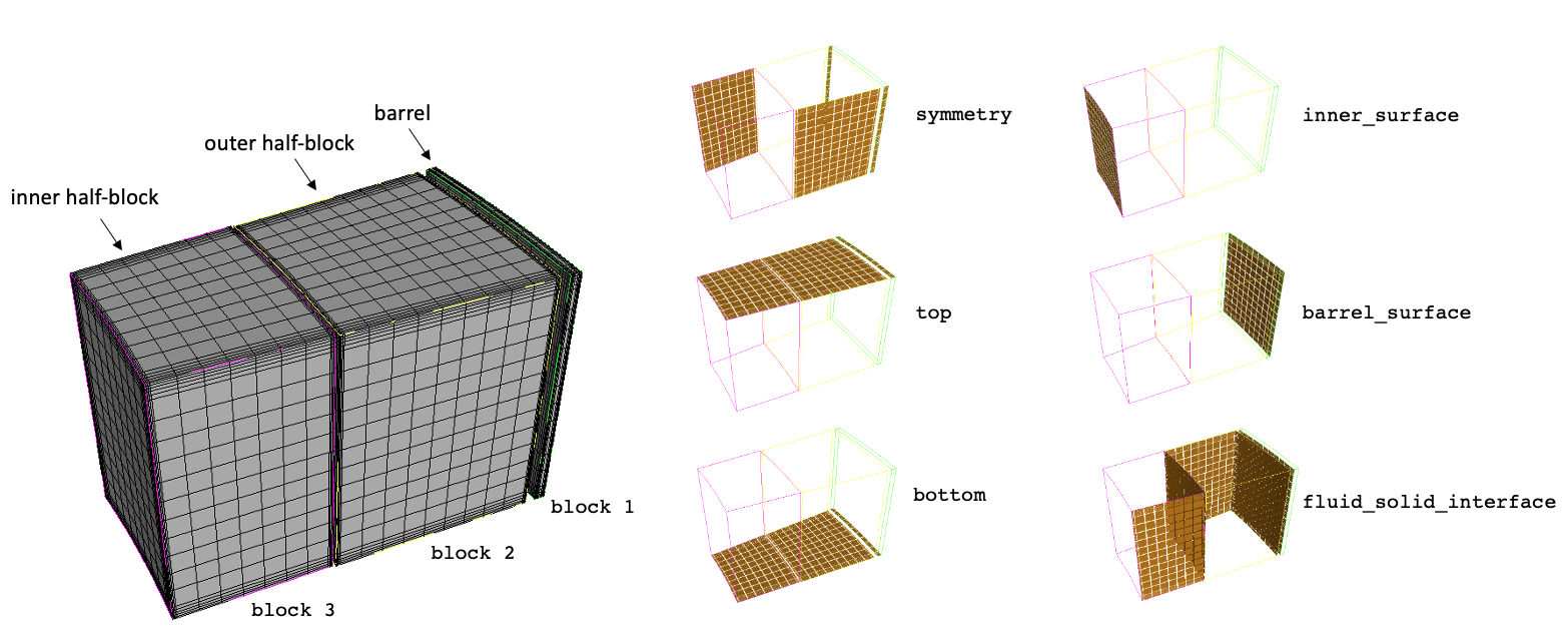
Figure 2: Solid mesh for the reflector blocks and barrel and a subset of the boundary names, before a series of mesh refinements

Unique boundary names are set for each boundary to which we will apply a unique boundary condition; we define the boundaries on the top and bottom of the block, the symmetry boundaries, and boundaries at the interface between the reflector and the bed and on the barrel surface.

One convenient aspect of MOOSE is that the same elements can be assigned to more than one boundary ID. To help in applying heat flux and temperature boundary conditions between NekRS and MOOSE, we define another boundary that contains all of the fluid-solid interfaces through which we will exchange heat flux and temperature, as fluid_solid_interface.

Fluid Mesh

The Cubit script used to generate the fluid mesh is shown below. To run this script yourself, you will need to update the directory variable to point to the tutorials directory on your machine.

#!python

# This is a mesh of 1/24th of the fluid in the outer reflector ring in the KP-FHR (there are 24
# blocks per ring). Only the fluid phase is modeled.

import math

# multiplicative factor to apply to the gap width; the nominal gap width cited
# in Shaver et. al (2019) corresponds to a gap amplification factor of 1.0.
gap_amplification = 3

# Path to the tutorials directory on your computer, if you want to run this script
# this will need to be updated
directory = '/Users/anovak/projects/cardinal/tutorials/'

core_radius       = 2.6
layer1_thickness  = 0.3
layer2_thickness  = 0.4
block_gap         = 0.002 * gap_amplification
bypass_gap        = 0.02
height            = 0.502
barrel_thickness  = 0.022
n_blocks_per_ring = 24
angle             = 360 / n_blocks_per_ring

barrel_outer_radius = core_radius + layer1_thickness + block_gap + layer2_thickness +\
  bypass_gap + barrel_thickness
barrel_inner_radius = barrel_outer_radius - barrel_thickness

layer2_outer_radius = barrel_inner_radius - bypass_gap
layer2_inner_radius = layer2_outer_radius - layer2_thickness

layer1_outer_radius = layer2_inner_radius - block_gap
layer1_inner_radius = layer1_outer_radius - layer1_thickness

porous_outer_radius = layer1_inner_radius
porous_inner_radius = porous_outer_radius - 3e-2

cubit.cmd('create cylinder radius ' + str(layer2_outer_radius) + ' height ' + str(height))
cubit.cmd('create cylinder radius ' + str(layer2_inner_radius) + ' height ' + str(height))
cubit.cmd('subtract volume 2 from volume 1')
cubit.cmd('compress all')
cubit.cmd('merge all')

cubit.cmd('create cylinder radius ' + str(layer1_outer_radius) + ' height ' + str(height))
cubit.cmd('create cylinder radius ' + str(layer1_inner_radius) + ' height ' + str(height))
cubit.cmd('subtract volume 3 from volume 2 keep')
cubit.cmd('delete volume 2')
cubit.cmd('compress all')
cubit.cmd('merge all')

# create the porous region
cubit.cmd('create cylinder radius ' + str(porous_inner_radius) + ' height ' + str(height))
cubit.cmd('subtract volume 4 from volume 2')
cubit.cmd('compress all')
cubit.cmd('merge all')

cubit.cmd('create brick x ' + str(2.0 * barrel_outer_radius) + ' y ' + str(barrel_outer_radius) + ' z ' + str(height))
cubit.cmd('move volume 4 y ' + str(-barrel_outer_radius / 2.0))
cubit.cmd('subtract volume 4 from volume 1 3')
cubit.cmd('compress all')
cubit.cmd('merge all')

cubit.cmd('create brick x ' + str(2.0 * barrel_outer_radius) + ' y ' + str(barrel_outer_radius) + ' z ' + str(height))
cubit.cmd('move volume 4 y ' + str(barrel_outer_radius / 2.0))
cubit.cmd('rotate volume 4 angle ' + str(angle) + ' about Z include_merged')
cubit.cmd('subtract volume 4 from volume 1 3')
cubit.cmd('compress all')
cubit.cmd('merge all')

cubit.cmd('create cylinder radius ' + str(barrel_outer_radius) + ' height ' + str(height))
cubit.cmd('create cylinder radius ' + str(barrel_inner_radius) + ' height ' + str(height))
cubit.cmd('subtract volume 5 from volume 4')
cubit.cmd('compress all')
cubit.cmd('merge all')

cubit.cmd('rotate Volume 1 angle ' + str(-angle / 2.0) + ' about origin 0 0 0 direction 0 0 1')

# create a block of fluid
cubit.cmd('create cylinder radius ' + str(barrel_outer_radius) + ' height ' + str(height))
cubit.cmd('create cylinder radius ' + str(layer1_inner_radius) + ' height ' + str(height))
cubit.cmd('subtract volume 6 from volume 5')
cubit.cmd('compress all')
cubit.cmd('merge all')

# size of gap between adjacent blocks in this model
l = block_gap / 2.0
cubit.cmd('create brick x ' + str(2.0 * barrel_outer_radius) + ' y ' + str(2.0 * barrel_outer_radius) + ' z ' + str(height))
cubit.cmd('move volume 6 y ' + str(-barrel_outer_radius - l))
cubit.cmd('subtract volume 6 from volume 2 4 5')
cubit.cmd('compress all')
cubit.cmd('merge all')

theta = (90.0 - angle / 2.0) * math.pi / 180.
cubit.cmd('create brick x ' + str(2.0 * barrel_outer_radius) + ' y ' + str(2.0 * barrel_outer_radius) + ' z ' + str(height))
cubit.cmd('move volume 6 y ' + str(barrel_outer_radius))
cubit.cmd('rotate volume 6 angle ' + str(angle / 2.0) + ' about Z include_merged')
cubit.cmd('move volume 6 x ' + str(-l * math.cos(theta)) + ' y ' + str(l * math.sin(theta)) + ' about Z include_merged')
cubit.cmd('subtract volume 6 from volume 2 4 5')
cubit.cmd('compress all')
cubit.cmd('merge all')

cubit.cmd('subtract volume 1 3 4 from volume 5')
cubit.cmd('compress all')
cubit.cmd('merge all')

cubit.cmd('subtract volume 2 from volume 1 imprint keep')
cubit.cmd('merge all')
cubit.cmd('compress all')
cubit.cmd('delete volume 1')
cubit.cmd('merge all')
cubit.cmd('compress all')

# now, create extra volumes just so that I have internal surfaces that I can
# use to control boundary layers
cubit.cmd('create brick x ' + str(2.0 * barrel_outer_radius) + ' y ' + str(2.0 * barrel_outer_radius) + ' z ' + str(height))
cubit.cmd('move volume 3 y ' + str(-barrel_outer_radius))
cubit.cmd('subtract volume 3 from volume 2 keep')
cubit.cmd('delete volume 3')
cubit.cmd('subtract volume 4 from volume 2 keep')
cubit.cmd('delete volume 2')
cubit.cmd('compress all')
cubit.cmd('merge all')

cubit.cmd('create cylinder radius ' + str(layer1_outer_radius) + ' height ' + str(height))
cubit.cmd('create cylinder radius ' + str(layer1_inner_radius) + ' height ' + str(height))
cubit.cmd('subtract volume 5 from volume 4')
cubit.cmd('compress all')
cubit.cmd('merge all')

cubit.cmd('subtract volume 4 from volume 1 imprint keep')
cubit.cmd('delete volume 4')
cubit.cmd('subtract volume 5 from volume 1 imprint keep')
cubit.cmd('delete volume 1')
cubit.cmd('compress all')
cubit.cmd('merge all')
cubit.cmd('imprint volume 1 2 3 4')

cubit.cmd('create cylinder radius ' + str(layer2_outer_radius) + ' height ' + str(height))
cubit.cmd('create cylinder radius ' + str(layer2_inner_radius) + ' height ' + str(height))
cubit.cmd('subtract volume 6 from volume 5')
cubit.cmd('compress all')
cubit.cmd('merge all')
cubit.cmd('subtract volume 5 from volume 3 keep')
cubit.cmd('delete volume 5')
cubit.cmd('split body 6')
cubit.cmd('subtract volume 6 7 from volume 3 keep')
cubit.cmd('delete volume 3')
cubit.cmd('compress all')
cubit.cmd('merge all')
cubit.cmd('imprint volume 1 2 3 4 5 6')

cubit.cmd('create cylinder radius ' + str(layer2_inner_radius) + ' height ' + str(height))
cubit.cmd('create cylinder radius ' + str(layer1_outer_radius) + ' height ' + str(height))
cubit.cmd('subtract volume 8 from volume 7')
cubit.cmd('create brick x ' + str(2.0 * barrel_outer_radius) + ' y ' + str(2.0 * barrel_outer_radius) + ' z ' + str(height))
cubit.cmd('move volume 9 y ' + str(-barrel_outer_radius))
cubit.cmd('subtract volume 9 from volume 7')
cubit.cmd('compress all')
cubit.cmd('merge all')

cubit.cmd('create brick x ' + str(2.0 * barrel_outer_radius) + ' y ' + str(2.0 * barrel_outer_radius) + ' z ' + str(height))
cubit.cmd('move volume 8 y ' + str(barrel_outer_radius))
cubit.cmd('rotate volume 8 angle ' + str(angle / 2.0) + ' about Z include_merged')
cubit.cmd('subtract volume 8 from volume 7 5 keep')
cubit.cmd('delete volume 8')
cubit.cmd('subtract volume 7 from volume 4 keep')
cubit.cmd('delete volume 7')
cubit.cmd('subtract volume 10 from volume 5 keep')
cubit.cmd('subtract volume 9 from volume 4 keep')
cubit.cmd('split body 13')
cubit.cmd('delete volume 4 5 14')
cubit.cmd('compress all')
cubit.cmd('merge all')
cubit.cmd('compress all')

cubit.cmd('delete volume 1 2')
cubit.cmd('merge all')
cubit.cmd('compress all')

cubit.cmd('block 1 volume 1 2 3 4 5 6 7')

surfaces = ''
for i in range(1, 36 + 1):
  surfaces += str(i) + ' '

cubit.cmd('surface ' + surfaces + ' size ' + str(block_gap))

gap_layer1 = 2e-4

# create boundary layers on all the surfaces - first, do the ones that naturally have corners
cubit.cmd('create boundary_layer 1')
cubit.cmd('modify boundary_layer 1 uniform height ' + str(gap_layer1) + ' growth 1.2 layers 4')
cubit.cmd('modify boundary_layer 1 add surface 23 volume 4 surface 30 volume 6')

cubit.cmd('create boundary_layer 2')
cubit.cmd('modify boundary_layer 2 uniform height ' + str(gap_layer1) + ' growth 1.2 layers 4')
cubit.cmd('modify boundary_layer 2 add surface 32 volume 6 surface 9 volume 2 surface 36 volume 7')

cubit.cmd('create boundary_layer 3')
cubit.cmd('modify boundary_layer 3 uniform height ' + str(gap_layer1) + ' growth 1.2 layers 4')
cubit.cmd('modify boundary_layer 3 add surface 28 volume 5 surface 6 volume 1')

# boundary layers on internal solid surfaces
cubit.cmd('create boundary_layer 5')
cubit.cmd('modify boundary_layer 5 uniform height ' + str(gap_layer1) + ' growth 1.2 layers 4')
cubit.cmd('modify boundary_layer 5 add surface 21 volume 4 surface 7 volume 6 surface 19 volume 6 surface 12 volume 2  surface 13 volume 7 surface 10 volume 7 surface 17 volume 3 surface 25 volume 5 surface 33 volume 7 surface 15 volume 3 surface 2 volume 5 surface 16 volume 5 surface 5 volume 1 surface 1 volume 1')

# "approach" boundary layers
cubit.cmd('create boundary_layer 6')
cubit.cmd('modify boundary_layer 6 uniform height ' + str(gap_layer1) + ' growth 1.6 layers ' + str(10 / uniform_refine))
cubit.cmd('modify boundary_layer 6 add surface 19 volume 4 surface 7 volume 2 surface 10 volume 2 surface 13 volume 3 surface 16 volume 3 surface 2 volume 1')

cubit.cmd('create boundary_layer 7')
cubit.cmd('modify boundary_layer 7 uniform height ' + str(gap_layer1 * 2) + ' growth 1.6 layers ' + str(6 / uniform_refine))
cubit.cmd('modify boundary_layer 7 add surface 4 volume 1 surface 11 volume 2 surface 18 volume 3 surface 20 volume 4 surface 26 volume 5 surface 31 volume 6 surface 34 volume 7')

cubit.cmd('create boundary_layer 8')
cubit.cmd('modify boundary_layer 8 uniform height ' + str(gap_layer1 * 2) + ' growth 1.6 layers ' + str(6 / uniform_refine))
cubit.cmd('modify boundary_layer 8 add surface 3 volume 1 surface 8 volume 2 surface 14 volume 3 surface 24 volume 4 surface 27 volume 5 surface 29 volume 6 surface 35 volume 7')

cubit.cmd('mesh volume 1 2 3 4 5 6 7')
cubit.cmd('block 1 element type HEX20')

# unite all the subblocks used just for the sake of controlling boundary layers
cubit.cmd('unite volume 1 2 3 4 5 6 7 include_mesh')
cubit.cmd('compress all')
cubit.cmd('merge all')

cubit.cmd('block 1 volume 1')

cubit.cmd('sideset 1 surface 7 5 9')
cubit.cmd('sideset 1 name "outer_block_surface"')

cubit.cmd('sideset 2 surface 2 6')
cubit.cmd('sideset 2 name "inner_block_surface"')

cubit.cmd('sideset 3 surface 3 10')
cubit.cmd('sideset 3 name "lower_symmetry"')

cubit.cmd('sideset 4 surface 4')
cubit.cmd('sideset 4 name "upper_symmetry"')

cubit.cmd('sideset 5 surface 8')
cubit.cmd('sideset 5 name "bottom_gaps"')

cubit.cmd('sideset 6 surface 12')
cubit.cmd('sideset 6 name "top_gaps"')

cubit.cmd('sideset 7 surface 11')
cubit.cmd('sideset 7 name "barrel_surface"')

cubit.cmd('sideset 8 surface 1')
cubit.cmd('sideset 8 name "porous_inner_surface"')

cubit.cmd('set large exodus file on')
cubit.cmd('export Genesis "' + directory + "fhr_reflector/meshes/" + 'fluid.exo" dimension 3 overwrite')

The fluid mesh is shown below; the boundary names are illustrated towards the right by showing the highlighted surface to which each boundary corresponds. While the names of the surfaces are shown, NekRS does not directly use these names - rather, NekRS assigns boundary conditions based on the boundary ID. An important restriction in NekRS is that the boundary IDs be ordered sequentially beginning from 1.

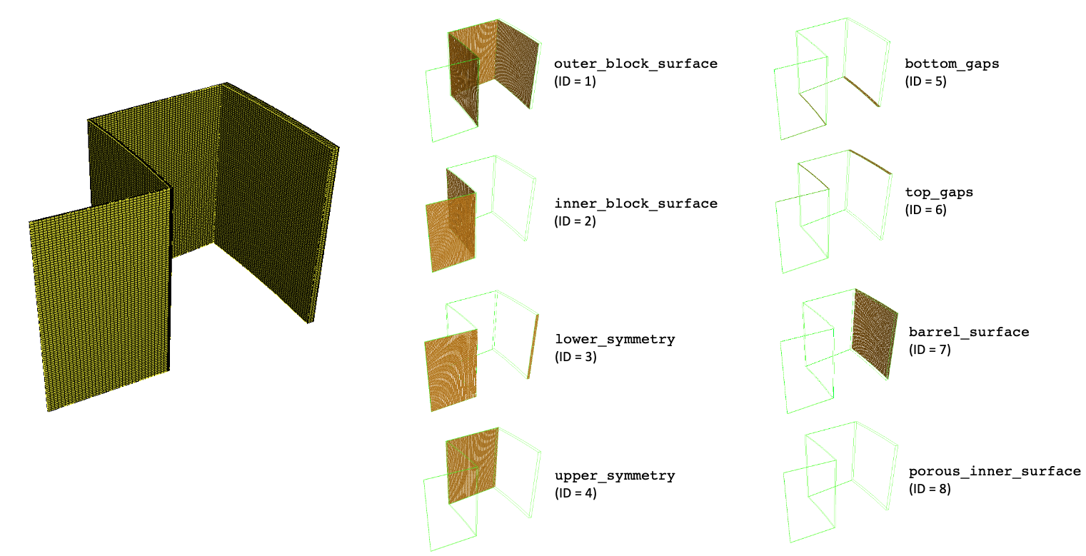
Fluid mesh for the FLiBe flowing around the reflector blocks, along with boundary names and IDs. It is difficult to see, but the `porous_inner_surface` boundary corresponds to the thin surface at the interface between the reflector region and the pebble bed.

Figure 3: Fluid mesh for the FLiBe flowing around the reflector blocks, along with boundary names and IDs. It is difficult to see, but the porous_inner_surface boundary corresponds to the thin surface at the interface between the reflector region and the pebble bed.

One strength of Cardinal for CHT applications is that the fluid and solid meshes do not need to share nodes on a common surface; MOOSE mesh-to-mesh data interpolations can communicate between surfaces with different refinement and position in space; meshes may even overlap or share no nodes at all, such as for curvilinear applications. Figure 4 shows a zoom-in of the two mesh files (for the fluid and solid phases). Each phase can be meshed according to its physics requirements.

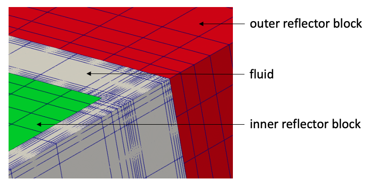
Figure 4: Zoomed-in view of the fluid and solid meshes, overlaid in Paraview. Lines are element boundaries.

Because NekRS uses a custom binary mesh format with a .re2 extension, the exo2nek utility must be used to convert an Exodus II format to .re2 format. For more information, please consult the tools documentation.

Part 1: Initial Conduction Coupling

In this section, NekRS and MOOSE are coupled for conduction heat transfer in the solid reflector blocks and barrel, and through a stagnant fluid. The purpose of this stage of the analysis is to obtain a restart file for use as an initial condition in Part 2: CHT Coupling to accelerate the NekRS calculation for CHT. All input files for this stage are present in the tutorials/fhr_reflector/conduction directory. The following sub-sections describe these files.

Solid Input Files

The solid phase is solved with the MOOSE heat transfer module, and is described in the solid.i input. At the top of this file, the core heat flux is defined as a variable local to the file.

# core average heat flux from the pebbles to the blocks
core_heat_flux = 5e3

Next, the solid mesh is specified by pointing to the Exodus mesh.

[Mesh<<<{"href": "../syntax/Mesh/index.html"}>>>]
  type = FileMesh
  file = ../meshes/solid.e
[]

The heat transfer module will solve for temperature, which is defined as a nonlinear variable.

[Variables<<<{"href": "../syntax/Variables/index.html"}>>>]
  [T]
  []
[]

The Transfer system is used to communicate auxiliary variables across applications; a boundary heat flux will be computed by MOOSE and applied as a boundary condition in NekRS. In the opposite direction, NekRS will compute a surface temperature that will be applied as a boundary condition in MOOSE. Therefore, both the flux (flux) and surface temperature (nek_temp) are declared as auxiliary variables. The solid app will compute flux, while nek_temp will simply receive a solution from NekRS.

[AuxVariables<<<{"href": "../syntax/AuxVariables/index.html"}>>>]
  [flux]
    family<<<{"description": "Specifies the family of FE shape functions to use for this variable"}>>> = MONOMIAL
    order<<<{"description": "Specifies the order of the FE shape function to use for this variable (additional orders not listed are allowed)"}>>> = CONSTANT
  []
  [nek_temp]
  []
[]

An initial condition is set for nek_temp using a function.

[Functions<<<{"href": "../syntax/Functions/index.html"}>>>]
  [nek_temp_ic]
    type = ParsedFunction<<<{"description": "Function created by parsing a string", "href": "../source/functions/MooseParsedFunction.html"}>>>
    expression<<<{"description": "The user defined function."}>>> = 923.0-50.0*(r-3.348)
    symbol_names<<<{"description": "Symbols (excluding t,x,y,z) that are bound to the values provided by the corresponding items in the vals vector."}>>> = 'r'
    symbol_values<<<{"description": "Constant numeric values, postprocessor names, function names, and scalar variables corresponding to the symbols in symbol_names."}>>> = 'r'
  []
  [r]
    type = ParsedFunction<<<{"description": "Function created by parsing a string", "href": "../source/functions/MooseParsedFunction.html"}>>>
    expression<<<{"description": "The user defined function."}>>> = sqrt(x*x+y*y)
  []
[]

[ICs<<<{"href": "../syntax/Cardinal/ICs/index.html"}>>>]
  [nek_temp]
    type = FunctionIC<<<{"description": "An initial condition that uses a normal function of x, y, z to produce values (and optionally gradients) for a field variable.", "href": "../source/ics/FunctionIC.html"}>>>
    variable<<<{"description": "The variable this initial condition is supposed to provide values for."}>>> = nek_temp
    function<<<{"description": "The initial condition function."}>>> = nek_temp_ic
  []
[]

Next, the governing equation solved by MOOSE is specified with the Kernels block.

[Kernels<<<{"href": "../syntax/Kernels/index.html"}>>>]
  [conduction]
    type = HeatConduction<<<{"description": "Diffusive heat conduction term $-\\nabla\\cdot(k\\nabla T)$ of the thermal energy conservation equation", "href": "../source/kernels/HeatConduction.html"}>>>
    variable<<<{"description": "The name of the variable that this residual object operates on"}>>> = T
  []
[]

[AuxKernels<<<{"href": "../syntax/AuxKernels/index.html"}>>>]
  [flux]
    type = DiffusionFluxAux<<<{"description": "Compute components of flux vector for diffusion problems $(\\vec{J} = -D \\nabla C)$.", "href": "../source/auxkernels/DiffusionFluxAux.html"}>>>
    variable<<<{"description": "The name of the variable that this object applies to"}>>> = flux
    diffusion_variable<<<{"description": "The name of the variable"}>>> = T
    component<<<{"description": "The desired component of flux."}>>> = normal
    check_boundary_restricted<<<{"description": "Whether to check for multiple element sides on the boundary in the case of a boundary restricted, element aux variable. Setting this to false will allow contribution to a single element's elemental value(s) from multiple boundary sides on the same element (example: when the restricted boundary exists on two or more sides of an element, such as at a corner of a mesh"}>>> = false
    diffusivity<<<{"description": "The name of the diffusivity material property that will be used in the flux computation."}>>> = thermal_conductivity
    boundary<<<{"description": "The list of boundaries (ids or names) from the mesh where this object applies"}>>> = 'fluid_solid_interface'
  []
[]

Next, the boundary conditions on the solid are applied. On the fluid-solid interface, a MatchedValueBC applies the value of the nek_temp receiver auxiliary variable to the temperature in a strong Dirichlet sense. Insulated boundary conditions are applied on the symmetry, top, and bottom boundaries. On the boundary at the bed-reflector interface, the core heat flux is specified as a NeumannBC. Finally, on the surface of the barrel, a heat flux of $var element = document.getElementById("moose-equation-518e590a-da4a-408a-ad84-cb73282318de");katex.render("h(T-T_\\infty)", element, {displayMode:false,throwOnError:false});$ is specified, where both $var element = document.getElementById("moose-equation-7501aae0-f00a-4b25-999d-4b7588a14ee2");katex.render("h", element, {displayMode:false,throwOnError:false});$ and $var element = document.getElementById("moose-equation-e8393a32-f14d-4de1-8c11-ddc5e6eaecf2");katex.render("T_\\infty", element, {displayMode:false,throwOnError:false});$ are specified as material properties.

[BCs<<<{"href": "../syntax/BCs/index.html"}>>>]
  [cht_interface]
    type = MatchedValueBC<<<{"description": "Implements a NodalBC which equates two different Variables' values on a specified boundary.", "href": "../source/bcs/MatchedValueBC.html"}>>>
    variable<<<{"description": "The name of the variable that this residual object operates on"}>>> = T
    v<<<{"description": "The variable whose value we are to match."}>>> = nek_temp
    boundary<<<{"description": "The list of boundary IDs from the mesh where this object applies"}>>> = 'fluid_solid_interface'
  []
  [insulated]
    type = NeumannBC<<<{"description": "Imposes the integrated boundary condition $\\frac{\\partial u}{\\partial n}=h$, where $h$ is a constant, controllable value.", "href": "../source/bcs/NeumannBC.html"}>>>
    variable<<<{"description": "The name of the variable that this residual object operates on"}>>> = T
    boundary<<<{"description": "The list of boundary IDs from the mesh where this object applies"}>>> = 'symmetry top bottom'
    value<<<{"description": "For a Laplacian problem, the value of the gradient dotted with the normals on the boundary."}>>> = 0.0
  []
  [inner_surface]
    type = NeumannBC<<<{"description": "Imposes the integrated boundary condition $\\frac{\\partial u}{\\partial n}=h$, where $h$ is a constant, controllable value.", "href": "../source/bcs/NeumannBC.html"}>>>
    variable<<<{"description": "The name of the variable that this residual object operates on"}>>> = T
    value<<<{"description": "For a Laplacian problem, the value of the gradient dotted with the normals on the boundary."}>>> = ${core_heat_flux}
    boundary<<<{"description": "The list of boundary IDs from the mesh where this object applies"}>>> = 'inner_surface'
  []
  [outer_surface]
    type = ConvectiveHeatFluxBC<<<{"description": "Convective heat transfer boundary condition with temperature and heat transfer coefficent given by material properties.", "href": "../source/bcs/ConvectiveHeatFluxBC.html"}>>>
    variable<<<{"description": "The name of the variable that this residual object operates on"}>>> = T
    T_infinity<<<{"description": "Material property for far-field temperature"}>>> = 'Tinf'
    heat_transfer_coefficient<<<{"description": "Material property for heat transfer coefficient"}>>> = 'htc'
    boundary<<<{"description": "The list of boundary IDs from the mesh where this object applies"}>>> = 'barrel_surface'
  []
[]

The HeatConduction kernel requires a material property for the thermal conductivity; material properties are also required for the heat transfer coefficient and far-field temperature for the ConvectiveHeatFluxBC boundary condition. These material properties are specified in the Materials block. Here, different values for thermal conductivity are used in the graphite and steel.

[Materials<<<{"href": "../syntax/Materials/index.html"}>>>]
  [k_graphite]
    type = GenericConstantMaterial<<<{"description": "Declares material properties based on names and values prescribed by input parameters.", "href": "../source/materials/GenericConstantMaterial.html"}>>>
    prop_names<<<{"description": "The names of the properties this material will have"}>>> = 'thermal_conductivity'
    prop_values<<<{"description": "The values associated with the named properties"}>>> = '43.73' # evaluated at 650 C
    block<<<{"description": "The list of blocks (ids or names) that this object will be applied"}>>> = '2 3'
  []
  [k_steel]
    type = GenericConstantMaterial<<<{"description": "Declares material properties based on names and values prescribed by input parameters.", "href": "../source/materials/GenericConstantMaterial.html"}>>>
    prop_names<<<{"description": "The names of the properties this material will have"}>>> = 'thermal_conductivity'
    prop_values<<<{"description": "The values associated with the named properties"}>>> = '23.82' # evaluated at 650 C
    block<<<{"description": "The list of blocks (ids or names) that this object will be applied"}>>> = '1'
  []
  [htc_and_Tinf]
    type = GenericConstantMaterial<<<{"description": "Declares material properties based on names and values prescribed by input parameters.", "href": "../source/materials/GenericConstantMaterial.html"}>>>
    prop_names<<<{"description": "The names of the properties this material will have"}>>> = 'htc Tinf'
    prop_values<<<{"description": "The values associated with the named properties"}>>> = '10.0 300.0'
  []
[]

Next, the MultiApps and Transfers blocks describe the interaction between Cardinal and MOOSE. The MOOSE heat transfer module is here run as the main application, with the NekRS wrapping run as the sub-application. We specify that MOOSE will run first on each time step.

Three transfers are required to couple Cardinal and MOOSE; the first is a transfer of surface temperature from Cardinal to MOOSE. The second is a transfer of heat flux from MOOSE to Cardinal. And the third is a transfer of the total integrated heat flux from MOOSE to Cardinal (computed as a postprocessor), which is then used internally by NekRS to re-normalize the heat flux (after interpolation onto NekRS's GLL points).

[MultiApps<<<{"href": "../syntax/MultiApps/index.html"}>>>]
  [nek]
    type = TransientMultiApp<<<{"description": "MultiApp for performing coupled simulations with the parent and sub-application both progressing in time.", "href": "../source/multiapps/TransientMultiApp.html"}>>>
    input_files<<<{"description": "The input file for each App.  If this parameter only contains one input file it will be used for all of the Apps.  When using 'positions_from_file' it is also admissable to provide one input_file per file."}>>> = 'nek.i'
    sub_cycling<<<{"description": "Set to true to allow this MultiApp to take smaller timesteps than the rest of the simulation.  More than one timestep will be performed for each parent application timestep"}>>> = true
    execute_on<<<{"description": "The list of flag(s) indicating when this object should be executed. For a description of each flag, see https://mooseframework.inl.gov/source/interfaces/SetupInterface.html."}>>> = timestep_end
  []
[]

[Transfers<<<{"href": "../syntax/Transfers/index.html"}>>>]
  [temperature_from_nek]
    type = MultiAppGeneralFieldNearestLocationTransfer<<<{"description": "Transfers field data at the MultiApp position by finding the value at the nearest neighbor(s) in the origin application.", "href": "../source/transfers/MultiAppGeneralFieldNearestLocationTransfer.html"}>>>
    source_variable<<<{"description": "The variable to transfer from."}>>> = temp
    from_multi_app<<<{"description": "The name of the MultiApp to receive data from"}>>> = nek
    variable<<<{"description": "The auxiliary variable to store the transferred values in."}>>> = nek_temp
  []
  [flux_to_nek]
    type = MultiAppGeneralFieldNearestLocationTransfer<<<{"description": "Transfers field data at the MultiApp position by finding the value at the nearest neighbor(s) in the origin application.", "href": "../source/transfers/MultiAppGeneralFieldNearestLocationTransfer.html"}>>>
    source_variable<<<{"description": "The variable to transfer from."}>>> = flux
    to_multi_app<<<{"description": "The name of the MultiApp to transfer the data to"}>>> = nek
    variable<<<{"description": "The auxiliary variable to store the transferred values in."}>>> = avg_flux
    from_boundaries<<<{"description": "The boundary we are transferring from (if not specified, whole domain is used)."}>>> = 'fluid_solid_interface'
  []
  [flux_integral_to_nek]
    type = MultiAppPostprocessorTransfer<<<{"description": "Transfers postprocessor data between the master application and sub-application(s).", "href": "../source/transfers/MultiAppPostprocessorTransfer.html"}>>>
    to_postprocessor<<<{"description": "The name of the Postprocessor in the MultiApp to transfer the value to.  This should most likely be a Reporter Postprocessor."}>>> = flux_integral
    from_postprocessor<<<{"description": "The name of the Postprocessor in the Master to transfer the value from."}>>> = flux_integral
    to_multi_app<<<{"description": "The name of the MultiApp to transfer the data to"}>>> = nek
  []
[]

Next, postprocessors are used to compute the integral heat flux as a SideIntegralVariablePostprocessor.

[Postprocessors<<<{"href": "../syntax/Postprocessors/index.html"}>>>]
  [flux_integral]
    type = SideIntegralVariablePostprocessor<<<{"description": "Computes a surface integral of the specified variable", "href": "../source/postprocessors/SideIntegralVariablePostprocessor.html"}>>>
    variable<<<{"description": "The name of the variable which this postprocessor integrates"}>>> = flux
    boundary<<<{"description": "The list of boundary IDs from the mesh where this object applies"}>>> = 'fluid_solid_interface'
  []
[]

Finally, a transient executioner is used for the solid phase. The overall coupled simulation is considered converged once the relative change in the solution between steps is less than $var element = document.getElementById("moose-equation-90758d80-3423-4031-a60f-1cb535c94ea1");katex.render("5\\times10^{-4}", element, {displayMode:false,throwOnError:false});$ . An output format of Exodus II is specified.

[Executioner<<<{"href": "../syntax/Executioner/index.html"}>>>]
  type = Transient
  dt = 0.005
  nl_abs_tol = 1e-6
  num_steps = 2000

  steady_state_detection = true
  steady_state_tolerance = 5e-4
[]

[Outputs<<<{"href": "../syntax/Outputs/index.html"}>>>]
  exodus<<<{"description": "Output the results using the default settings for Exodus output."}>>> = true
  print_linear_residuals<<<{"description": "Enable printing of linear residuals to the screen (Console)"}>>> = false
[]

Fluid Input Files

The fluid phase is solved with NekRS. The wrapping of NekRS as a MOOSE application is specified in the nek.i file.

First, a local variable, fluid_solid_interface, is used to define all the boundary IDs through which NekRS is coupled via CHT to MOOSE. A first-order mirror of the NekRS mesh is constructed using the NekRSMesh. By specifying the boundary parameter, we are indicating that NekRS will be coupled via CHT through boundaries 1, 2, and 7 to MOOSE. In order for MOOSE's transfers to correctly find the closest nodes in the solid mesh to corresponding nodes in this fluid mesh mirror, the entire mesh must be scaled by a factor of $var element = document.getElementById("moose-equation-75fcf341-ab34-496b-b83e-30432b5d3efa");katex.render("L_{ref}", element, {displayMode:false,throwOnError:false});$ to return to dimensional units (because the coupled MOOSE application is in dimensional units). This scaling is specified by the scaling parameter.

fluid_solid_interface = '1 2 7'

[Mesh<<<{"href": "../syntax/Mesh/index.html"}>>>]
  type = NekRSMesh
  boundary = ${fluid_solid_interface}
  scaling = 0.006
[]

Next, the NekRSProblem specifies that NekRS simulations will be run in place of MOOSE. To allow conversion between a non-dimensional NekRS solve and a dimensional MOOSE coupled heat conduction application, the characteristic scales used to establish the non-dimensional problem are provided. The wall heat flux will be written into NekRS using a NekBoundaryFlux object; this automatically creates an auxiliary variable named avg_flux and a Receiver postprocessor named flux_integral. A NekFieldVariable is used to read out temperature into an auxiliary variable (created automatically) named temp.

[Problem<<<{"href": "../syntax/Problem/index.html"}>>>]
  type = NekRSProblem
  casename<<<{"description": "Case name for the NekRS input files; this is <case> in <case>.par, <case>.udf, <case>.oudf, and <case>.re2."}>>> = 'fluid'
  n_usrwrk_slots<<<{"description": "Number of slots to allocate in nrs->usrwrk to hold fields either related to coupling (which will be populated by Cardinal), or other custom usages, such as a distance-to-wall calculation"}>>> = 1

  [FieldTransfers<<<{"href": "../syntax/Problem/FieldTransfers/index.html"}>>>]
    [avg_flux]
      type = NekBoundaryFlux<<<{"description": "Reads/writes boundary flux data between NekRS and MOOSE."}>>>
      direction<<<{"description": "Direction in which to send data"}>>> = to_nek
      usrwrk_slot<<<{"description": "When 'direction = to_nek', the slot(s) in the usrwrk array to write the incoming data; provide one entry for each quantity being passed"}>>> = 0
      postprocessor_to_conserve<<<{"description": "Name of the postprocessor/vectorpostprocessor containing the integral(s) used to ensure conservation; defaults to the name of the object plus '_integral'"}>>> = flux_integral
    []
    [temp]
      type = NekFieldVariable<<<{"description": "Reads/writes volumetric field data between NekRS and MOOSE."}>>>
      direction<<<{"description": "Direction in which to send data"}>>> = from_nek
      field<<<{"description": "NekRS field variable to read/write; defaults to the name of the object"}>>> = temperature
    []
  []

  [Dimensionalize<<<{"href": "../syntax/Problem/Dimensionalize/index.html"}>>>]
    U<<<{"description": "Reference velocity"}>>> = 0.0575
    T<<<{"description": "Reference temperature"}>>> = 923.15
    dT<<<{"description": "Reference temperature difference"}>>> = 10.0
    L<<<{"description": "Reference length"}>>> = 0.006
    rho<<<{"description": "Reference density"}>>> = 1962.13
    Cp<<<{"description": "Reference isobaric specific heat"}>>> = 2416.0
  []
[]

Next, a Transient executioner is specified with the NekTimeStepper, which allows NekRS to control its own time stepping (except for synchronization points).

[Executioner<<<{"href": "../syntax/Executioner/index.html"}>>>]
  type = Transient

  [TimeStepper<<<{"href": "../syntax/Executioner/TimeStepper/index.html"}>>>]
    type = NekTimeStepper
  []
[]

[Outputs<<<{"href": "../syntax/Outputs/index.html"}>>>]
  exodus<<<{"description": "Output the results using the default settings for Exodus output."}>>> = true
[]

Finally, several postprocessors are included to perform integrals and global min/max calculations over the NekRS domain for diagnostic purposes. Here, the NekHeatFluxIntegral postprocessor computes $var element = document.getElementById("moose-equation-650070d7-2b41-4992-8a2a-e783c79b954e");katex.render("-k\\nabla T\\cdot\\hat{n}", element, {displayMode:false,throwOnError:false});$ over a boundary in the NekRS mesh. The NekVolumeExtremeValue postprocessors then compute the maximum and minimum temperatures throughout the entire NekRS domain (i.e. not only on the CHT coupling surfaces).

[Postprocessors<<<{"href": "../syntax/Postprocessors/index.html"}>>>]
  [boundary_flux]
    type = NekHeatFluxIntegral<<<{"description": "Heat flux over a boundary in the NekRS mesh", "href": "../source/postprocessors/NekHeatFluxIntegral.html"}>>>
    boundary<<<{"description": "Boundary ID(s) for which to compute the postprocessor"}>>> = ${fluid_solid_interface}
  []
  [max_nek_T]
    type = NekVolumeExtremeValue<<<{"description": "Extreme value (max/min) of a field over the NekRS mesh", "href": "../source/postprocessors/NekVolumeExtremeValue.html"}>>>
    field<<<{"description": "Field to apply this object to"}>>> = temperature
    value_type<<<{"description": "Whether to give the maximum or minimum extreme value"}>>> = max
  []
  [min_nek_T]
    type = NekVolumeExtremeValue<<<{"description": "Extreme value (max/min) of a field over the NekRS mesh", "href": "../source/postprocessors/NekVolumeExtremeValue.html"}>>>
    field<<<{"description": "Field to apply this object to"}>>> = temperature
    value_type<<<{"description": "Whether to give the maximum or minimum extreme value"}>>> = min
  []
[]

The nek.i input file only describes how NekRS is wrapped within the MOOSE framework; each NekRS simulation requires additional files that share the same case name fluid but with different extensions. The additional NekRS files are:

fluid.re2: Mesh file
fluid.par: High-level settings for the solver, boundary condition mappings to sidesets, and the equations to solve
fluid.udf: User-defined C++ functions for on-line postprocessing and model setup
fluid.oudf: User-defined OCCA kernels for boundary conditions and source terms

First, begin with the fluid.par file.

# Input of solid conduction through FLiBe in the outer reflector block fluid region.
# Material properties are taken for FLiBe at 650 C.

# The problem is run in nondimensional form with the following characteristic scales:
# L_ref  = 0.006    (the width of the smallest block-block gap)
# V_ref  = 0.0575   (velocity needed to get the specified Reynolds number)
# T_ref  = 923.15   (the inlet temperature)
# dT_ref = 10.0     (arbitrary temperature range value)
# t_ref  = 0.1043   (reference time scale)
# rho_0  = 1962.13
# mu_0   = 6.77e-3
# Cp_0   = 2416
# k_0    = 1.09
# Pr     = 15.005

[GENERAL]
  stopAt = numSteps
  numSteps = 2000
  dt = 0.025
  timeStepper = tombo2
  writeControl = steps
  writeInterval = 100
  polynomialOrder = 2

[VELOCITY]
  solver = none

[PRESSURE]

[TEMPERATURE]
  conductivity = -1500.5
  rhoCp = 1.0
  residualTol = 1.0e-8
  boundaryTypeMap = f, f, I, I, t, o, f, I

Here, a time step of 0.025 (non-dimensional) is used; a NekRS output file is written every 100 time steps. Because the purpose of this simulation is only to obtain a reasonable initial condition, a low polynomial order of 2 is used.

Next, the [VELOCITY] and [PRESSURE] blocks describe the solution of the pressure Poisson equation and velocity Helmholtz equations. In the velocity block, setting solver = none turns off the velocity solution; therefore, none of the parameters specified here are used right now, so their description will be deferred to Part 2: CHT Coupling . Finally, the [TEMPERATURE] block describes the solution of the temperature passive scalar equation. $var element = document.getElementById("moose-equation-6b4a4a43-5c5b-446a-839f-6ad3ac070e40");katex.render("\\rho_fC_{p,f}", element, {displayMode:false,throwOnError:false});$ is set to unity because the solve is conducted in non-dimensional form, such that

$(3)var element = document.getElementById("moose-equation-c0820d19-6d4c-41e3-86b7-45e73a7483cf");katex.render(" \\rho^\\dagger C_{p,f}^\\dagger\\equiv\\frac{\\rho_fC_{p,f}}{\\rho_0C_{p,0}}=1", element, {displayMode:true,throwOnError:false});$

The coefficient on the diffusive equation term in the non-dimensional energy equation is equal to $var element = document.getElementById("moose-equation-13ea4ee3-9182-4b7a-9413-bc80436480d3");katex.render("1/Pe", element, {displayMode:false,throwOnError:false});$ . In NekRS, specifying conductivity = -1500.5 is equivalent to specifying conductivity = 0.00066644 (i.e. $var element = document.getElementById("moose-equation-48ee6f5e-8b80-4d42-881a-39eeaeb6b858");katex.render("1/1500.5", element, {displayMode:false,throwOnError:false});$ ), or a Peclet number of 1500.5.

Next, residualTol specifies the solver tolerance for the temperature equation to $var element = document.getElementById("moose-equation-a79af886-35cf-42ad-a29d-e15d30a31d60");katex.render("10^{-8}", element, {displayMode:false,throwOnError:false});$ . Finally, the boundaryTypeMap is used to specify the mapping of boundary IDs to types of boundary conditions. Boundaries 1, 2, and 7 are flux boundaries (these boundaries will receive a heat flux from MOOSE), boundaries 3, 4, and 8 are insulated, boundary 5 is a specified temperature, and boundary 6 is a zero-gradient outlet. The actual assignment of values for these boundary conditions is then performed in the fluid.oudf file. Because this case does not have any user-defined source terms in NekRS, these OCCA kernels are only used to apply boundary conditions.

void scalarDirichletConditions(bcData * bc)
{
  if (bc->id == 5)
    bc->s = 0.0;
}

void scalarNeumannConditions(bcData * bc)
{
  // note: when running with Cardinal, Cardinal will allocate the usrwrk
  // array. If running with NekRS standalone (e.g. nrsmpi), you need to
  // replace the usrwrk with some other value or allocate it youself from
  // the udf and populate it with values.
  if (bc->id == 1 || bc->id == 2 || bc->id == 7)
    bc->flux = bc->usrwrk[bc->idM];
}

Finally, the fluid.udf file contains user-defined C++ functions through which other interactions with the NekRS solution are performed. Here, the UDF_Setup function is called once at the very start of the NekRS simulation, and it is here that initial conditions are applied.

#include "udf.hpp"

void UDF_LoadKernels(occa::properties & kernelInfo)
{
}

void UDF_Setup(nrs_t *nrs)
{
  mesh_t * mesh = nrs->cds->mesh[0];

  // loop over all the GLL points and assign directly to the solution arrays by
  // indexing according to the field offset necessary to hold the data for each
  // solution component
  int n_gll_points = mesh->Np * mesh->Nelements;
  for (int n = 0; n < n_gll_points; ++n)
    nrs->cds->S[n] = 0;
}

The initial condition is applied by looping over all the GLL points and setting zero to each (recall that this is a non-dimensional simulation, such that $var element = document.getElementById("moose-equation-97a91c88-2255-4024-856c-eb3262f8618e");katex.render("T^\\dagger=0", element, {displayMode:false,throwOnError:false});$ corresponds to a dimensional temperature of $var element = document.getElementById("moose-equation-d0b49db0-8aac-48b0-b27c-2c9928ad3a82");katex.render("T_{ref}", element, {displayMode:false,throwOnError:false});$ ). Here, nrs->cds->S is the array holding the NekRS passive scalar solutions (of which there is only one for this example).

Execution and Postprocessing

To run the pseudo-steady conduction model, run the following:


mpiexec -np 48 cardinal-opt -i solid.i

which will run with 48 MPI ranks. When the simulation has completed, you will have created a number of different output files:

fluid0.f<n>, where <n> is a five-digit number indicating the output file number created by NekRS (a separate output file is written for each time step according to the settings in the fluid.par file). An extra program is required to visualize NekRS output files in Paraview; see the instructions here.
solid_out.e, an Exodus II output file with the solid mesh and solution.
solid_out_nek0.e, an Exodus II output file with the fluid mirror mesh and data that was ultimately transferred in/out of NekRS.

After converting the NekRS output files to a format viewable in Paraview, the simulation results can be displayed. The solid temperature, surface heat flux, and fluid temperature are shown below. Note that the fluid temperature is shown in nondimensional form based on the selected characteristic scales. The image of the fluid solution is rotated so as to better display the temperature variation around the inner reflector block. The domain shown in Figure 6 exactly corresponds to the "mirror" mesh constructed by NekRSMesh.

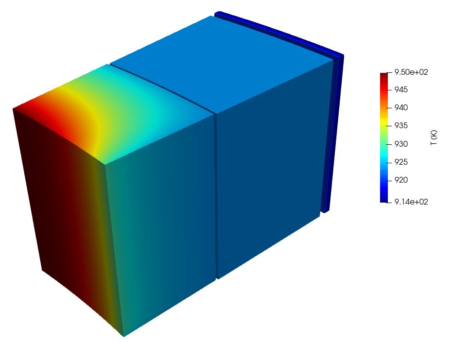
Figure 5: Solid temperature for steady state conduction coupling between MOOSE and NekRS

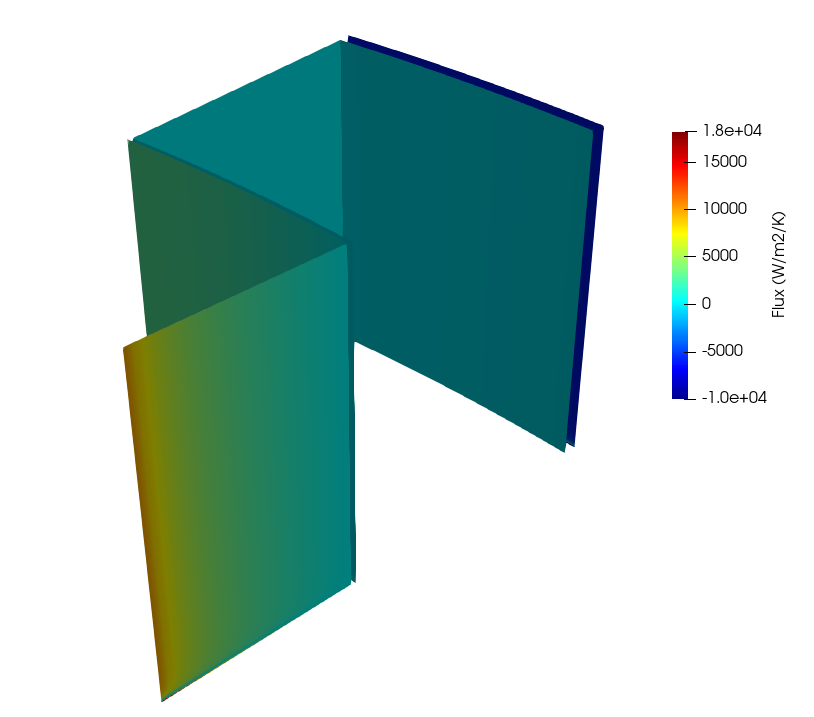
Figure 6: Solid surface heat flux for steady state conduction coupling between MOOSE and NekRS

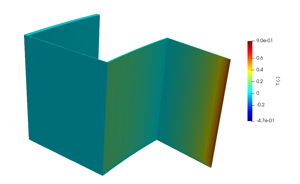
Figure 7: Fluid temperature (nondimensional) for steady state conduction coupling between MOOSE and NekRS

The solid blocks are heated by the pebble bed along the bed-reflector interface, so the temperatures are highest in the inner block. As can be seen in Figure 6, the heat flux into the fluid is in some places positive (such as near the inner reflector block) and is in other places negative (such as near the barrel) where heat leaves the system.

Part 2: CHT Coupling

In this section, NekRS and MOOSE are coupled for CHT with fluid flow. All input files for this stage of the analysis are present in the tutorials/fhr_reflector/cht directory. The following sub-sections describe all of these files; for brevity, most emphasis will be placed on input file setup that is different or extends the conduction case in Part 1: Initial Conduction Coupling .

Solid Input Files

The solid phase is again solved with the MOOSE heat transfer module; the input file is largely the same except that the simulation is run for 400 time steps.

[Executioner<<<{"href": "../syntax/Executioner/index.html"}>>>]
  type = Transient
  dt = 0.001
  nl_abs_tol = 1e-5
  l_max_its = 100
  num_steps = 400
[]

Fluid Input Files

The fluid phase is solved with NekRS. The input file is largely the same as the conduction case, except that additional postprocessors are added to query more aspects of the NekRS solution. The postprocessors are shown below.

[Postprocessors<<<{"href": "../syntax/Postprocessors/index.html"}>>>]
  [boundary_flux]
    type = NekHeatFluxIntegral<<<{"description": "Heat flux over a boundary in the NekRS mesh", "href": "../source/postprocessors/NekHeatFluxIntegral.html"}>>>
    boundary<<<{"description": "Boundary ID(s) for which to compute the postprocessor"}>>> = ${fluid_solid_interface}
  []
  [max_nek_T]
    type = NekVolumeExtremeValue<<<{"description": "Extreme value (max/min) of a field over the NekRS mesh", "href": "../source/postprocessors/NekVolumeExtremeValue.html"}>>>
    field<<<{"description": "Field to apply this object to"}>>> = temperature
    value_type<<<{"description": "Whether to give the maximum or minimum extreme value"}>>> = max
  []
  [min_nek_T]
    type = NekVolumeExtremeValue<<<{"description": "Extreme value (max/min) of a field over the NekRS mesh", "href": "../source/postprocessors/NekVolumeExtremeValue.html"}>>>
    field<<<{"description": "Field to apply this object to"}>>> = temperature
    value_type<<<{"description": "Whether to give the maximum or minimum extreme value"}>>> = min
  []
  [pressure_in]
    type = NekSideAverage<<<{"description": "Average of a field over a boundary of the NekRS mesh", "href": "../source/postprocessors/NekSideAverage.html"}>>>
    field<<<{"description": "Field to apply this object to"}>>> = pressure
    boundary<<<{"description": "Boundary ID(s) for which to compute the postprocessor"}>>> = '5'
  []
  [mdot_in]
    type = NekMassFluxWeightedSideIntegral<<<{"description": "Mass flux weighted integral of a field over a boundary of the NekRS mesh", "href": "../source/postprocessors/NekMassFluxWeightedSideIntegral.html"}>>>
    field<<<{"description": "Field to apply this object to"}>>> = unity
    boundary<<<{"description": "Boundary ID(s) for which to compute the postprocessor"}>>> = '5'
  []
  [mdot_out]
    type = NekMassFluxWeightedSideIntegral<<<{"description": "Mass flux weighted integral of a field over a boundary of the NekRS mesh", "href": "../source/postprocessors/NekMassFluxWeightedSideIntegral.html"}>>>
    field<<<{"description": "Field to apply this object to"}>>> = unity
    boundary<<<{"description": "Boundary ID(s) for which to compute the postprocessor"}>>> = '6'
  []
[]

We have added postprocessors to compute the average inlet pressure and the average inlet and outlet mass flowrates. Like the NekVolumeExtremeValue postprocessor, these postprocessors operate directly on NekRS's internal solution arrays to provide diagnostic information. Because the outlet pressure is set to zero, pressure_in corresponds to the pressure drop in the fluid.

As in Part 1: Initial Conduction Coupling , additional files are required to set up the NekRS simulation - fluid.re2, fluid.par, fluid.udf, and fluid.oudf. These files are largely the same as those used in the steady conduction model, so only the differences will be emphasized here. The fluid.par file is shown below. Here, startFrom provides a restart file (that we generated from Part 1: Initial Conduction Coupling ), conduction.fld and specifies that we only want to read temperature from the file (by appending +T to the file name). We increase the polynomial order as well.

# Input of fluid flow of FLiBe in the outer reflector block fluid region.
# Material properties are taken for FLiBe at 650 C.

# The problem is run in nondimensional form with the following characteristic scales:
# L_ref  = 0.006    (the width of the smallest block-block gap)
# V_ref  = 0.0575   (velocity needed to get the specified Reynolds number)
# T_ref  = 923.15   (the inlet temperature)
# dT_ref = 10.0     (arbitrary temperature range value)
# t_ref  = 0.0208   (reference time scale)
# rho_0  = 1962.13
# mu_0   = 6.77e-3
# Cp_0   = 2416
# k_0    = 1.09
# Pr     = 15.005

[GENERAL]
  startFrom = conduction.fld+T
  stopAt = numSteps
  numSteps = 2000
  dt = 0.001
  timeStepper = tombo2
  writeControl = steps
  writeInterval = 100
  polynomialOrder = 4

[VELOCITY]
  viscosity = -100.0
  density = 1.0
  residualTol = 1.0e-8
  boundaryTypeMap = W, W, symy, W, v, o, W, W

[PRESSURE]
  residualTol = 1.0e-8

[TEMPERATURE]
  conductivity = -1500.5
  rhoCp = 1.0
  residualTol = 1.0e-8
  boundaryTypeMap = f, f, I, I, t, o, f, I

In the [VELOCITY] block, the density is set to unity, because the solve is conducted in nondimensional form, such that

$(4)var element = document.getElementById("moose-equation-9d091a9f-09a7-44c8-a7da-a7c33e40210c");katex.render(" \\rho^\\dagger\\equiv\\frac{\\rho_f}{\\rho_0}=1", element, {displayMode:true,throwOnError:false});$

The coefficient on the diffusive term in the non-dimensional momentum equation is equal to $var element = document.getElementById("moose-equation-ed0e0730-e7fc-4d07-81a2-a79401464e55");katex.render("1/Re", element, {displayMode:false,throwOnError:false});$ . In NekRS, specifying diffusivity = -100.0 is equivalent to specifying diffusivity = 0.001 (i.e. $var element = document.getElementById("moose-equation-efa21860-9bc4-49a4-90a0-85a8652026a3");katex.render("1/100.0", element, {displayMode:false,throwOnError:false});$ ), or a Reynolds number of 100.0. All other parameters have similar interpretations as described in Part 1: Initial Conduction Coupling .

The fluid.udf file is shown below. The UDF_Setup function is again used to apply initial conditions; because temperature is read from the restart file, only initial conditions on velocity and pressure are required. nrs->U is an array storing the three components of velocity (padded with length nrs->fieldOffset), while nrs->P is the array storing the pressure solution.

#include "udf.hpp"

void UDF_LoadKernels(occa::properties & kernelInfo)
{
  // Compute the inlet velocity boundary condition and propagate it to a kernel variable
  kernelInfo["defines/Vz"] = 1.0;

  // Compute the inlet temperature and propagate it to a kernel variable
  kernelInfo["defines/inlet_T"] = 0.0;
}

void UDF_Setup(nrs_t *nrs)
{
  mesh_t * mesh = nrs->cds->mesh[0];

  // loop over all the GLL points and assign directly to the solution arrays by
  // indexing according to the field offset necessary to hold the data for each
  // solution component
  int n_gll_points = mesh->Np * mesh->Nelements;
  for (int n = 0; n < n_gll_points; ++n)
  {
    nrs->U[n + 0 * nrs->fieldOffset] = 0.0; // x-velocity
    nrs->U[n + 1 * nrs->fieldOffset] = 0.0; // y-velocity
    nrs->U[n + 2 * nrs->fieldOffset] = 1.0; // z-velocity

    nrs->P[n] = 0.0; // pressure
  }
}

This file also includes the UDF_LoadKernels function, which is used to propagate quantities to variables accessible through OCCA kernels. The kernelInfo object is used to define two variables - Vz and inlet_T that will be accessible through the GPU kernels, eliminating some burden on the user if the problem setup must be changed in multiple locations throughout the NekRS input files.

Finally, the fluid.oudf file is shown below. Because the velocity is enabled, additional boundary condition functions must be specified. In the velocityDirichletConditions function, the kernel variable Vz was defined in the fluid.udf file. The other boundary conditions - the Dirichlet temperature conditions and the Neumann heat flux conditions - are the same as for the steady conduction case.

void velocityDirichletConditions(bcData * bc)
{
  if (bc->id == 5)
  {
    bc->u = 0.0; // x-velocity
    bc->v = 0.0; // y-velocity
    bc->w = Vz;  // z-velocity
  }
}

void scalarDirichletConditions(bcData * bc)
{
  if (bc->id == 5)
    bc->s = inlet_T;
}

void scalarNeumannConditions(bcData * bc)
{
  // note: when running with Cardinal, Cardinal will allocate the usrwrk
  // array. If running with NekRS standalone (e.g. nrsmpi), you need to
  // replace the usrwrk with some other value or allocate it youself from
  // the udf and populate it with values.
  if (bc->id == 1 || bc->id == 2 | bc->id == 7)
    bc->flux = bc->usrwrk[bc->idM];
}

Execution and Postprocessing

To run the pseudo-steady CHT model, run the following:


$ mpiexec -np 48 cardinal-opt -i solid.i

The pressure and velocity distributions are shown below, both in non-dimensional form.

Pressure (nondimensional) for [!ac](CHT) coupling between MOOSE and NekRS

Figure 8: Pressure (nondimensional) for CHT coupling between MOOSE and NekRS

Velocity (nondimensional) for [!ac](CHT) coupling between MOOSE and NekRS

Figure 9: Velocity (nondimensional) for CHT coupling between MOOSE and NekRS

The no-slip condition on the solid surface, and the symmetry condition on the $var element = document.getElementById("moose-equation-80e9d1ff-f330-4c99-a82d-c9cc9b6bc3d7");katex.render("y=0", element, {displayMode:false,throwOnError:false});$ surface, are clear in Figure 9. The pressure loss is highest in the gap along the $var element = document.getElementById("moose-equation-d228848b-1c42-4885-a99c-07bf9467ef4d");katex.render("\\theta=7.5^\\circ", element, {displayMode:false,throwOnError:false});$ boundary due to the imposition of no-slip conditions on both sides of the half-gap width.

References

A.J. Novak, S. Schunert, R.W. Carlsen, P. Balestra, R.N. Slaybaugh, and R.C. Martineau. Multiscale thermal-hydraulic modeling of the pebble bed fluoride-salt-cooled high-temperature reactor. Annals of Nuclear Energy, 2021. doi:10.1016/j.anucene.2020.107968.

@article{novak2021,
    author = "Novak, A.J. and Schunert, S. and Carlsen, R.W. and Balestra, P. and Slaybaugh, R.N. and Martineau, R.C.",
    title = "Multiscale Thermal-Hydraulic Modeling of the Pebble Bed Fluoride-Salt-Cooled High-Temperature Reactor",
    doi = "10.1016/j.anucene.2020.107968",
    journal = "Annals of Nuclear Energy",
    year = "2021",
    volume = "154"
}

A.J. Novak, D. Shaver, and B. Feng. Conjugate Heat Transfer Coupling of NekRS and MOOSE for Bypass Flow Modeling. In Proceedings of ANS. 2021.

@InProceedings{novak_ans_2021,
    author = "Novak, A.J. and Shaver, D. and Feng, B.",
    title = "{Conjugate Heat Transfer Coupling of NekRS and MOOSE for Bypass Flow Modeling}",
    booktitle = "{Proceedings of ANS}",
    year = "2021"
}

D. Shaver, R. Hu, L. Zou, and E. Merzari. Initial Industry Collaborations of the Center of Excellence. Technical Report ANL/NSE-19/15, Argonne National Laboratory, 2019. URL: https://www.osti.gov/biblio/1556071.

@TechReport{shaver,
    author = "Shaver, D. and Hu, R. and Zou, L. and Merzari, E.",
    title = "{Initial Industry Collaborations of the Center of Excellence}",
    institution = "Argonne National Laboratory",
    year = "2019",
    number = "ANL/NSE-19/15",
    url = "https://www.osti.gov/biblio/1556071"
}

SNL. CUBIT 13.2 User Documentation. 2012. URL: https://tinyurl.com/rgsbqb7.

(tutorials/fhr_reflector/meshes/solid.jou)

#!python

# This is a mesh of half of 1/24th of the outer reflector ring in a pebble bed
# fluoride-salt-cooled high temperature reactor (there are 24
# blocks per ring), in addition to the barrel. Only the solid phase is modeled.

import math

# multiplicative factor to apply to the gap width; the nominal gap width cited
# in Shaver et. al (2019) corresponds to a gap amplification factor of 1.0.
gap_amplification = 3

# Path to the tutorials directory on your computer, if you want to run this script
# this will need to be updated
directory = '/Users/anovak/projects/cardinal/tutorials/'

core_radius       = 2.6
layer1_thickness  = 0.3
layer2_thickness  = 0.4
block_gap         = 0.002 * gap_amplification
bypass_gap        = 0.02
height            = 0.502
barrel_thickness  = 0.022
n_blocks_per_ring = 24
angle             = 360 / n_blocks_per_ring

barrel_outer_radius = core_radius + layer1_thickness + block_gap + layer2_thickness +\
                      bypass_gap + barrel_thickness

barrel_inner_radius = barrel_outer_radius - barrel_thickness

layer2_outer_radius = barrel_inner_radius - bypass_gap

layer2_inner_radius = layer2_outer_radius - layer2_thickness

layer1_outer_radius = layer2_inner_radius - block_gap

layer1_inner_radius = layer1_outer_radius - layer1_thickness

cubit.cmd('create cylinder radius ' + str(barrel_outer_radius) + ' height ' + str(height))
cubit.cmd('create cylinder radius ' + str(barrel_inner_radius) + ' height ' + str(height))
cubit.cmd('subtract volume 2 from volume 1')
cubit.cmd('compress all')
cubit.cmd('merge all')

cubit.cmd('create cylinder radius ' + str(layer2_outer_radius) + ' height ' + str(height))
cubit.cmd('create cylinder radius ' + str(layer2_inner_radius) + ' height ' + str(height))
cubit.cmd('subtract volume 3 from volume 2')
cubit.cmd('compress all')
cubit.cmd('merge all')

cubit.cmd('create cylinder radius ' + str(layer1_outer_radius) + ' height ' + str(height))
cubit.cmd('create cylinder radius ' + str(layer1_inner_radius) + ' height ' + str(height))
cubit.cmd('subtract volume 4 from volume 3')
cubit.cmd('compress all')
cubit.cmd('merge all')

l = block_gap / 2.0
cubit.cmd('create brick x ' + str(2.0 * barrel_outer_radius) + ' y ' + str(2.0 * barrel_outer_radius) + ' z ' + str(height))
cubit.cmd('move volume 4 y ' + str(-barrel_outer_radius - l))
cubit.cmd('subtract volume 4 from volume 1 2')
cubit.cmd('compress all')
cubit.cmd('merge all')

cubit.cmd('create brick x ' + str(2.0 * barrel_outer_radius) + ' y ' + str(barrel_outer_radius) + ' z ' + str(height))
cubit.cmd('move volume 4 y ' + str(-barrel_outer_radius / 2.0))
cubit.cmd('subtract volume 4 from volume 3')
cubit.cmd('compress all')
cubit.cmd('merge all')

theta = (90.0 - angle / 2.0) * math.pi / 180.
cubit.cmd('create brick x ' + str(2.0 * barrel_outer_radius) + ' y ' + str(2.0 * barrel_outer_radius) + ' z ' + str(height))
cubit.cmd('move volume 4 y ' + str(barrel_outer_radius))
cubit.cmd('rotate volume 4 angle ' + str(angle / 2.0) + ' about Z include_merged')
cubit.cmd('move volume 4 x ' + str(-l * math.cos(theta)) + ' y ' + str(l * math.sin(theta)) + ' about Z include_merged')
cubit.cmd('subtract volume 4 from volume 3 1')
cubit.cmd('compress all')
cubit.cmd('merge all')

cubit.cmd('create brick x ' + str(2.0 * barrel_outer_radius) + ' y ' + str(barrel_outer_radius) + ' z ' + str(height))
cubit.cmd('move volume 4 y ' + str(barrel_outer_radius / 2.0))
cubit.cmd('rotate volume 4 angle ' + str(angle / 2.0) + ' about Z include_merged')
cubit.cmd('subtract volume 4 from volume 2')
cubit.cmd('compress all')
cubit.cmd('merge all')

cubit.cmd('block 1 volume 1')
cubit.cmd('block 2 volume 2')
cubit.cmd('block 3 volume 3')

# create boundary layers on all the surfaces
cubit.cmd('create boundary_layer 1')
cubit.cmd('modify boundary_layer 1 uniform height 3e-3 growth 1.2 layers 4')
cubit.cmd('modify boundary_layer 1 add surface 1 volume 1 surface 2 volume 2 surface 3 volume 3')

cubit.cmd('create boundary_layer 2')
cubit.cmd('modify boundary_layer 2 uniform height 3e-3 growth 1.2 layers 4')
cubit.cmd('modify boundary_layer 2 add surface 9 volume 1 surface 14 volume 2 surface 4 volume 3')

cubit.cmd('create boundary_layer 3')
cubit.cmd('modify boundary_layer 3 uniform height 2e-3 growth 1.2 layers 8')
cubit.cmd('modify boundary_layer 3 add surface 10 volume 1 surface 15 volume 2 surface 5 volume 3')

cubit.cmd('create boundary_layer 4')
cubit.cmd('modify boundary_layer 4 uniform height 2e-3 growth 1.2 layers 8')
cubit.cmd('modify boundary_layer 4 add surface 13 volume 1 surface 18 volume 2 surface 8 volume 3')

cubit.cmd('create boundary_layer 5')
cubit.cmd('modify boundary_layer 5 uniform height 1.5e-3 growth 1.2 layers 4')
cubit.cmd('modify boundary_layer 5 add surface 12 volume 1 surface 11 volume 1 surface 17 volume 2 surface 16 volume 2 surface 7 volume 3 surface 6 volume 3')

size_division = 50

cubit.cmd('volume 1 2 3 size ' + str(layer1_thickness / size_division))

cubit.cmd('mesh volume 1 2 3')
cubit.cmd('block 1 2 3 element type HEX8')

cubit.cmd('sideset 1 surface 1 2 4 9')
cubit.cmd('sideset 1 name "symmetry"')

cubit.cmd('sideset 3 surface 8 13 18')
cubit.cmd('sideset 3 name "bottom"')

cubit.cmd('sideset 4 surface 5 10 15')
cubit.cmd('sideset 4 name "top"')

cubit.cmd('sideset 5 surface 6')
cubit.cmd('sideset 5 name "inner_surface"')

cubit.cmd('sideset 6 surface 12')
cubit.cmd('sideset 6 name "barrel_surface"')

cubit.cmd('sideset 100 surface 3 7 16 14 17 11')
cubit.cmd('sideset 100 name "fluid_solid_interface"')

cubit.cmd('set large exodus file on')
cubit.cmd('export Genesis "' + directory + 'fhr_reflector/meshes/solid.e" dimension 3 overwrite')

(tutorials/fhr_reflector/meshes/fluid.jou)

#!python

# This is a mesh of 1/24th of the fluid in the outer reflector ring in the KP-FHR (there are 24
# blocks per ring). Only the fluid phase is modeled.

import math

# multiplicative factor to apply to the gap width; the nominal gap width cited
# in Shaver et. al (2019) corresponds to a gap amplification factor of 1.0.
gap_amplification = 3

# Path to the tutorials directory on your computer, if you want to run this script
# this will need to be updated
directory = '/Users/anovak/projects/cardinal/tutorials/'

core_radius       = 2.6
layer1_thickness  = 0.3
layer2_thickness  = 0.4
block_gap         = 0.002 * gap_amplification
bypass_gap        = 0.02
height            = 0.502
barrel_thickness  = 0.022
n_blocks_per_ring = 24
angle             = 360 / n_blocks_per_ring

barrel_outer_radius = core_radius + layer1_thickness + block_gap + layer2_thickness +\
  bypass_gap + barrel_thickness
barrel_inner_radius = barrel_outer_radius - barrel_thickness

layer2_outer_radius = barrel_inner_radius - bypass_gap
layer2_inner_radius = layer2_outer_radius - layer2_thickness

layer1_outer_radius = layer2_inner_radius - block_gap
layer1_inner_radius = layer1_outer_radius - layer1_thickness

porous_outer_radius = layer1_inner_radius
porous_inner_radius = porous_outer_radius - 3e-2

cubit.cmd('create cylinder radius ' + str(layer2_outer_radius) + ' height ' + str(height))
cubit.cmd('create cylinder radius ' + str(layer2_inner_radius) + ' height ' + str(height))
cubit.cmd('subtract volume 2 from volume 1')
cubit.cmd('compress all')
cubit.cmd('merge all')

cubit.cmd('create cylinder radius ' + str(layer1_outer_radius) + ' height ' + str(height))
cubit.cmd('create cylinder radius ' + str(layer1_inner_radius) + ' height ' + str(height))
cubit.cmd('subtract volume 3 from volume 2 keep')
cubit.cmd('delete volume 2')
cubit.cmd('compress all')
cubit.cmd('merge all')

# create the porous region
cubit.cmd('create cylinder radius ' + str(porous_inner_radius) + ' height ' + str(height))
cubit.cmd('subtract volume 4 from volume 2')
cubit.cmd('compress all')
cubit.cmd('merge all')

cubit.cmd('create brick x ' + str(2.0 * barrel_outer_radius) + ' y ' + str(barrel_outer_radius) + ' z ' + str(height))
cubit.cmd('move volume 4 y ' + str(-barrel_outer_radius / 2.0))
cubit.cmd('subtract volume 4 from volume 1 3')
cubit.cmd('compress all')
cubit.cmd('merge all')

cubit.cmd('create brick x ' + str(2.0 * barrel_outer_radius) + ' y ' + str(barrel_outer_radius) + ' z ' + str(height))
cubit.cmd('move volume 4 y ' + str(barrel_outer_radius / 2.0))
cubit.cmd('rotate volume 4 angle ' + str(angle) + ' about Z include_merged')
cubit.cmd('subtract volume 4 from volume 1 3')
cubit.cmd('compress all')
cubit.cmd('merge all')

cubit.cmd('create cylinder radius ' + str(barrel_outer_radius) + ' height ' + str(height))
cubit.cmd('create cylinder radius ' + str(barrel_inner_radius) + ' height ' + str(height))
cubit.cmd('subtract volume 5 from volume 4')
cubit.cmd('compress all')
cubit.cmd('merge all')

cubit.cmd('rotate Volume 1 angle ' + str(-angle / 2.0) + ' about origin 0 0 0 direction 0 0 1')

# create a block of fluid
cubit.cmd('create cylinder radius ' + str(barrel_outer_radius) + ' height ' + str(height))
cubit.cmd('create cylinder radius ' + str(layer1_inner_radius) + ' height ' + str(height))
cubit.cmd('subtract volume 6 from volume 5')
cubit.cmd('compress all')
cubit.cmd('merge all')

# size of gap between adjacent blocks in this model
l = block_gap / 2.0
cubit.cmd('create brick x ' + str(2.0 * barrel_outer_radius) + ' y ' + str(2.0 * barrel_outer_radius) + ' z ' + str(height))
cubit.cmd('move volume 6 y ' + str(-barrel_outer_radius - l))
cubit.cmd('subtract volume 6 from volume 2 4 5')
cubit.cmd('compress all')
cubit.cmd('merge all')

theta = (90.0 - angle / 2.0) * math.pi / 180.
cubit.cmd('create brick x ' + str(2.0 * barrel_outer_radius) + ' y ' + str(2.0 * barrel_outer_radius) + ' z ' + str(height))
cubit.cmd('move volume 6 y ' + str(barrel_outer_radius))
cubit.cmd('rotate volume 6 angle ' + str(angle / 2.0) + ' about Z include_merged')
cubit.cmd('move volume 6 x ' + str(-l * math.cos(theta)) + ' y ' + str(l * math.sin(theta)) + ' about Z include_merged')
cubit.cmd('subtract volume 6 from volume 2 4 5')
cubit.cmd('compress all')
cubit.cmd('merge all')

cubit.cmd('subtract volume 1 3 4 from volume 5')
cubit.cmd('compress all')
cubit.cmd('merge all')

cubit.cmd('subtract volume 2 from volume 1 imprint keep')
cubit.cmd('merge all')
cubit.cmd('compress all')
cubit.cmd('delete volume 1')
cubit.cmd('merge all')
cubit.cmd('compress all')

# now, create extra volumes just so that I have internal surfaces that I can
# use to control boundary layers
cubit.cmd('create brick x ' + str(2.0 * barrel_outer_radius) + ' y ' + str(2.0 * barrel_outer_radius) + ' z ' + str(height))
cubit.cmd('move volume 3 y ' + str(-barrel_outer_radius))
cubit.cmd('subtract volume 3 from volume 2 keep')
cubit.cmd('delete volume 3')
cubit.cmd('subtract volume 4 from volume 2 keep')
cubit.cmd('delete volume 2')
cubit.cmd('compress all')
cubit.cmd('merge all')

cubit.cmd('create cylinder radius ' + str(layer1_outer_radius) + ' height ' + str(height))
cubit.cmd('create cylinder radius ' + str(layer1_inner_radius) + ' height ' + str(height))
cubit.cmd('subtract volume 5 from volume 4')
cubit.cmd('compress all')
cubit.cmd('merge all')

cubit.cmd('subtract volume 4 from volume 1 imprint keep')
cubit.cmd('delete volume 4')
cubit.cmd('subtract volume 5 from volume 1 imprint keep')
cubit.cmd('delete volume 1')
cubit.cmd('compress all')
cubit.cmd('merge all')
cubit.cmd('imprint volume 1 2 3 4')

cubit.cmd('create cylinder radius ' + str(layer2_outer_radius) + ' height ' + str(height))
cubit.cmd('create cylinder radius ' + str(layer2_inner_radius) + ' height ' + str(height))
cubit.cmd('subtract volume 6 from volume 5')
cubit.cmd('compress all')
cubit.cmd('merge all')
cubit.cmd('subtract volume 5 from volume 3 keep')
cubit.cmd('delete volume 5')
cubit.cmd('split body 6')
cubit.cmd('subtract volume 6 7 from volume 3 keep')
cubit.cmd('delete volume 3')
cubit.cmd('compress all')
cubit.cmd('merge all')
cubit.cmd('imprint volume 1 2 3 4 5 6')

cubit.cmd('create cylinder radius ' + str(layer2_inner_radius) + ' height ' + str(height))
cubit.cmd('create cylinder radius ' + str(layer1_outer_radius) + ' height ' + str(height))
cubit.cmd('subtract volume 8 from volume 7')
cubit.cmd('create brick x ' + str(2.0 * barrel_outer_radius) + ' y ' + str(2.0 * barrel_outer_radius) + ' z ' + str(height))
cubit.cmd('move volume 9 y ' + str(-barrel_outer_radius))
cubit.cmd('subtract volume 9 from volume 7')
cubit.cmd('compress all')
cubit.cmd('merge all')

cubit.cmd('create brick x ' + str(2.0 * barrel_outer_radius) + ' y ' + str(2.0 * barrel_outer_radius) + ' z ' + str(height))
cubit.cmd('move volume 8 y ' + str(barrel_outer_radius))
cubit.cmd('rotate volume 8 angle ' + str(angle / 2.0) + ' about Z include_merged')
cubit.cmd('subtract volume 8 from volume 7 5 keep')
cubit.cmd('delete volume 8')
cubit.cmd('subtract volume 7 from volume 4 keep')
cubit.cmd('delete volume 7')
cubit.cmd('subtract volume 10 from volume 5 keep')
cubit.cmd('subtract volume 9 from volume 4 keep')
cubit.cmd('split body 13')
cubit.cmd('delete volume 4 5 14')
cubit.cmd('compress all')
cubit.cmd('merge all')
cubit.cmd('compress all')

cubit.cmd('delete volume 1 2')
cubit.cmd('merge all')
cubit.cmd('compress all')

cubit.cmd('block 1 volume 1 2 3 4 5 6 7')

surfaces = ''
for i in range(1, 36 + 1):
  surfaces += str(i) + ' '

cubit.cmd('surface ' + surfaces + ' size ' + str(block_gap))

gap_layer1 = 2e-4

# create boundary layers on all the surfaces - first, do the ones that naturally have corners
cubit.cmd('create boundary_layer 1')
cubit.cmd('modify boundary_layer 1 uniform height ' + str(gap_layer1) + ' growth 1.2 layers 4')
cubit.cmd('modify boundary_layer 1 add surface 23 volume 4 surface 30 volume 6')

cubit.cmd('create boundary_layer 2')
cubit.cmd('modify boundary_layer 2 uniform height ' + str(gap_layer1) + ' growth 1.2 layers 4')
cubit.cmd('modify boundary_layer 2 add surface 32 volume 6 surface 9 volume 2 surface 36 volume 7')

cubit.cmd('create boundary_layer 3')
cubit.cmd('modify boundary_layer 3 uniform height ' + str(gap_layer1) + ' growth 1.2 layers 4')
cubit.cmd('modify boundary_layer 3 add surface 28 volume 5 surface 6 volume 1')

# boundary layers on internal solid surfaces
cubit.cmd('create boundary_layer 5')
cubit.cmd('modify boundary_layer 5 uniform height ' + str(gap_layer1) + ' growth 1.2 layers 4')
cubit.cmd('modify boundary_layer 5 add surface 21 volume 4 surface 7 volume 6 surface 19 volume 6 surface 12 volume 2  surface 13 volume 7 surface 10 volume 7 surface 17 volume 3 surface 25 volume 5 surface 33 volume 7 surface 15 volume 3 surface 2 volume 5 surface 16 volume 5 surface 5 volume 1 surface 1 volume 1')

# "approach" boundary layers
cubit.cmd('create boundary_layer 6')
cubit.cmd('modify boundary_layer 6 uniform height ' + str(gap_layer1) + ' growth 1.6 layers ' + str(10 / uniform_refine))
cubit.cmd('modify boundary_layer 6 add surface 19 volume 4 surface 7 volume 2 surface 10 volume 2 surface 13 volume 3 surface 16 volume 3 surface 2 volume 1')

cubit.cmd('create boundary_layer 7')
cubit.cmd('modify boundary_layer 7 uniform height ' + str(gap_layer1 * 2) + ' growth 1.6 layers ' + str(6 / uniform_refine))
cubit.cmd('modify boundary_layer 7 add surface 4 volume 1 surface 11 volume 2 surface 18 volume 3 surface 20 volume 4 surface 26 volume 5 surface 31 volume 6 surface 34 volume 7')

cubit.cmd('create boundary_layer 8')
cubit.cmd('modify boundary_layer 8 uniform height ' + str(gap_layer1 * 2) + ' growth 1.6 layers ' + str(6 / uniform_refine))
cubit.cmd('modify boundary_layer 8 add surface 3 volume 1 surface 8 volume 2 surface 14 volume 3 surface 24 volume 4 surface 27 volume 5 surface 29 volume 6 surface 35 volume 7')

cubit.cmd('mesh volume 1 2 3 4 5 6 7')
cubit.cmd('block 1 element type HEX20')

# unite all the subblocks used just for the sake of controlling boundary layers
cubit.cmd('unite volume 1 2 3 4 5 6 7 include_mesh')
cubit.cmd('compress all')
cubit.cmd('merge all')

cubit.cmd('block 1 volume 1')

cubit.cmd('sideset 1 surface 7 5 9')
cubit.cmd('sideset 1 name "outer_block_surface"')

cubit.cmd('sideset 2 surface 2 6')
cubit.cmd('sideset 2 name "inner_block_surface"')

cubit.cmd('sideset 3 surface 3 10')
cubit.cmd('sideset 3 name "lower_symmetry"')

cubit.cmd('sideset 4 surface 4')
cubit.cmd('sideset 4 name "upper_symmetry"')

cubit.cmd('sideset 5 surface 8')
cubit.cmd('sideset 5 name "bottom_gaps"')

cubit.cmd('sideset 6 surface 12')
cubit.cmd('sideset 6 name "top_gaps"')

cubit.cmd('sideset 7 surface 11')
cubit.cmd('sideset 7 name "barrel_surface"')

cubit.cmd('sideset 8 surface 1')
cubit.cmd('sideset 8 name "porous_inner_surface"')

cubit.cmd('set large exodus file on')
cubit.cmd('export Genesis "' + directory + "fhr_reflector/meshes/" + 'fluid.exo" dimension 3 overwrite')

(tutorials/fhr_reflector/conduction/solid.i)

# core average heat flux from the pebbles to the blocks
core_heat_flux = 5e3

[Mesh]
  type = FileMesh
  file = ../meshes/solid.e
[]

[Variables]
  [T]
  []
[]

[AuxVariables]
  [flux]
    family = MONOMIAL
    order = CONSTANT
  []
  [nek_temp]
  []
[]

[Functions]
  [nek_temp_ic]
    type = ParsedFunction
    expression = 923.0-50.0*(r-3.348)
    symbol_names = 'r'
    symbol_values = 'r'
  []
  [r]
    type = ParsedFunction
    expression = sqrt(x*x+y*y)
  []
[]

[ICs]
  [nek_temp]
    type = FunctionIC
    variable = nek_temp
    function = nek_temp_ic
  []
[]

[Kernels]
  [conduction]
    type = HeatConduction
    variable = T
  []
[]

[AuxKernels]
  [flux]
    type = DiffusionFluxAux
    variable = flux
    diffusion_variable = T
    component = normal
    check_boundary_restricted = false
    diffusivity = thermal_conductivity
    boundary = 'fluid_solid_interface'
  []
[]

[BCs]
  [cht_interface]
    type = MatchedValueBC
    variable = T
    v = nek_temp
    boundary = 'fluid_solid_interface'
  []
  [insulated]
    type = NeumannBC
    variable = T
    boundary = 'symmetry top bottom'
    value = 0.0
  []
  [inner_surface]
    type = NeumannBC
    variable = T
    value = ${core_heat_flux}
    boundary = 'inner_surface'
  []
  [outer_surface]
    type = ConvectiveHeatFluxBC
    variable = T
    T_infinity = 'Tinf'
    heat_transfer_coefficient = 'htc'
    boundary = 'barrel_surface'
  []
[]

[Materials]
  [k_graphite]
    type = GenericConstantMaterial
    prop_names = 'thermal_conductivity'
    prop_values = '43.73' # evaluated at 650 C
    block = '2 3'
  []
  [k_steel]
    type = GenericConstantMaterial
    prop_names = 'thermal_conductivity'
    prop_values = '23.82' # evaluated at 650 C
    block = '1'
  []
  [htc_and_Tinf]
    type = GenericConstantMaterial
    prop_names = 'htc Tinf'
    prop_values = '10.0 300.0'
  []
[]

[MultiApps]
  [nek]
    type = TransientMultiApp
    input_files = 'nek.i'
    sub_cycling = true
    execute_on = timestep_end
  []
[]

[Transfers]
  [temperature_from_nek]
    type = MultiAppGeneralFieldNearestLocationTransfer
    source_variable = temp
    from_multi_app = nek
    variable = nek_temp
  []
  [flux_to_nek]
    type = MultiAppGeneralFieldNearestLocationTransfer
    source_variable = flux
    to_multi_app = nek
    variable = avg_flux
    from_boundaries = 'fluid_solid_interface'
  []
  [flux_integral_to_nek]
    type = MultiAppPostprocessorTransfer
    to_postprocessor = flux_integral
    from_postprocessor = flux_integral
    to_multi_app = nek
  []
[]

[Postprocessors]
  [flux_integral]
    type = SideIntegralVariablePostprocessor
    variable = flux
    boundary = 'fluid_solid_interface'
  []
[]

[Executioner]
  type = Transient
  dt = 0.005
  nl_abs_tol = 1e-6
  num_steps = 2000

  steady_state_detection = true
  steady_state_tolerance = 5e-4
[]

[Outputs]
  exodus = true
  print_linear_residuals = false
[]

(tutorials/fhr_reflector/conduction/solid.i)

# core average heat flux from the pebbles to the blocks
core_heat_flux = 5e3

[Mesh]
  type = FileMesh
  file = ../meshes/solid.e
[]

[Variables]
  [T]
  []
[]

[AuxVariables]
  [flux]
    family = MONOMIAL
    order = CONSTANT
  []
  [nek_temp]
  []
[]

[Functions]
  [nek_temp_ic]
    type = ParsedFunction
    expression = 923.0-50.0*(r-3.348)
    symbol_names = 'r'
    symbol_values = 'r'
  []
  [r]
    type = ParsedFunction
    expression = sqrt(x*x+y*y)
  []
[]

[ICs]
  [nek_temp]
    type = FunctionIC
    variable = nek_temp
    function = nek_temp_ic
  []
[]

[Kernels]
  [conduction]
    type = HeatConduction
    variable = T
  []
[]

[AuxKernels]
  [flux]
    type = DiffusionFluxAux
    variable = flux
    diffusion_variable = T
    component = normal
    check_boundary_restricted = false
    diffusivity = thermal_conductivity
    boundary = 'fluid_solid_interface'
  []
[]

[BCs]
  [cht_interface]
    type = MatchedValueBC
    variable = T
    v = nek_temp
    boundary = 'fluid_solid_interface'
  []
  [insulated]
    type = NeumannBC
    variable = T
    boundary = 'symmetry top bottom'
    value = 0.0
  []
  [inner_surface]
    type = NeumannBC
    variable = T
    value = ${core_heat_flux}
    boundary = 'inner_surface'
  []
  [outer_surface]
    type = ConvectiveHeatFluxBC
    variable = T
    T_infinity = 'Tinf'
    heat_transfer_coefficient = 'htc'
    boundary = 'barrel_surface'
  []
[]

[Materials]
  [k_graphite]
    type = GenericConstantMaterial
    prop_names = 'thermal_conductivity'
    prop_values = '43.73' # evaluated at 650 C
    block = '2 3'
  []
  [k_steel]
    type = GenericConstantMaterial
    prop_names = 'thermal_conductivity'
    prop_values = '23.82' # evaluated at 650 C
    block = '1'
  []
  [htc_and_Tinf]
    type = GenericConstantMaterial
    prop_names = 'htc Tinf'
    prop_values = '10.0 300.0'
  []
[]

[MultiApps]
  [nek]
    type = TransientMultiApp
    input_files = 'nek.i'
    sub_cycling = true
    execute_on = timestep_end
  []
[]

[Transfers]
  [temperature_from_nek]
    type = MultiAppGeneralFieldNearestLocationTransfer
    source_variable = temp
    from_multi_app = nek
    variable = nek_temp
  []
  [flux_to_nek]
    type = MultiAppGeneralFieldNearestLocationTransfer
    source_variable = flux
    to_multi_app = nek
    variable = avg_flux
    from_boundaries = 'fluid_solid_interface'
  []
  [flux_integral_to_nek]
    type = MultiAppPostprocessorTransfer
    to_postprocessor = flux_integral
    from_postprocessor = flux_integral
    to_multi_app = nek
  []
[]

[Postprocessors]
  [flux_integral]
    type = SideIntegralVariablePostprocessor
    variable = flux
    boundary = 'fluid_solid_interface'
  []
[]

[Executioner]
  type = Transient
  dt = 0.005
  nl_abs_tol = 1e-6
  num_steps = 2000

  steady_state_detection = true
  steady_state_tolerance = 5e-4
[]

[Outputs]
  exodus = true
  print_linear_residuals = false
[]

(tutorials/fhr_reflector/conduction/solid.i)

# core average heat flux from the pebbles to the blocks
core_heat_flux = 5e3

[Mesh]
  type = FileMesh
  file = ../meshes/solid.e
[]

[Variables]
  [T]
  []
[]

[AuxVariables]
  [flux]
    family = MONOMIAL
    order = CONSTANT
  []
  [nek_temp]
  []
[]

[Functions]
  [nek_temp_ic]
    type = ParsedFunction
    expression = 923.0-50.0*(r-3.348)
    symbol_names = 'r'
    symbol_values = 'r'
  []
  [r]
    type = ParsedFunction
    expression = sqrt(x*x+y*y)
  []
[]

[ICs]
  [nek_temp]
    type = FunctionIC
    variable = nek_temp
    function = nek_temp_ic
  []
[]

[Kernels]
  [conduction]
    type = HeatConduction
    variable = T
  []
[]

[AuxKernels]
  [flux]
    type = DiffusionFluxAux
    variable = flux
    diffusion_variable = T
    component = normal
    check_boundary_restricted = false
    diffusivity = thermal_conductivity
    boundary = 'fluid_solid_interface'
  []
[]

[BCs]
  [cht_interface]
    type = MatchedValueBC
    variable = T
    v = nek_temp
    boundary = 'fluid_solid_interface'
  []
  [insulated]
    type = NeumannBC
    variable = T
    boundary = 'symmetry top bottom'
    value = 0.0
  []
  [inner_surface]
    type = NeumannBC
    variable = T
    value = ${core_heat_flux}
    boundary = 'inner_surface'
  []
  [outer_surface]
    type = ConvectiveHeatFluxBC
    variable = T
    T_infinity = 'Tinf'
    heat_transfer_coefficient = 'htc'
    boundary = 'barrel_surface'
  []
[]

[Materials]
  [k_graphite]
    type = GenericConstantMaterial
    prop_names = 'thermal_conductivity'
    prop_values = '43.73' # evaluated at 650 C
    block = '2 3'
  []
  [k_steel]
    type = GenericConstantMaterial
    prop_names = 'thermal_conductivity'
    prop_values = '23.82' # evaluated at 650 C
    block = '1'
  []
  [htc_and_Tinf]
    type = GenericConstantMaterial
    prop_names = 'htc Tinf'
    prop_values = '10.0 300.0'
  []
[]

[MultiApps]
  [nek]
    type = TransientMultiApp
    input_files = 'nek.i'
    sub_cycling = true
    execute_on = timestep_end
  []
[]

[Transfers]
  [temperature_from_nek]
    type = MultiAppGeneralFieldNearestLocationTransfer
    source_variable = temp
    from_multi_app = nek
    variable = nek_temp
  []
  [flux_to_nek]
    type = MultiAppGeneralFieldNearestLocationTransfer
    source_variable = flux
    to_multi_app = nek
    variable = avg_flux
    from_boundaries = 'fluid_solid_interface'
  []
  [flux_integral_to_nek]
    type = MultiAppPostprocessorTransfer
    to_postprocessor = flux_integral
    from_postprocessor = flux_integral
    to_multi_app = nek
  []
[]

[Postprocessors]
  [flux_integral]
    type = SideIntegralVariablePostprocessor
    variable = flux
    boundary = 'fluid_solid_interface'
  []
[]

[Executioner]
  type = Transient
  dt = 0.005
  nl_abs_tol = 1e-6
  num_steps = 2000

  steady_state_detection = true
  steady_state_tolerance = 5e-4
[]

[Outputs]
  exodus = true
  print_linear_residuals = false
[]

(tutorials/fhr_reflector/conduction/solid.i)

# core average heat flux from the pebbles to the blocks
core_heat_flux = 5e3

[Mesh]
  type = FileMesh
  file = ../meshes/solid.e
[]

[Variables]
  [T]
  []
[]

[AuxVariables]
  [flux]
    family = MONOMIAL
    order = CONSTANT
  []
  [nek_temp]
  []
[]

[Functions]
  [nek_temp_ic]
    type = ParsedFunction
    expression = 923.0-50.0*(r-3.348)
    symbol_names = 'r'
    symbol_values = 'r'
  []
  [r]
    type = ParsedFunction
    expression = sqrt(x*x+y*y)
  []
[]

[ICs]
  [nek_temp]
    type = FunctionIC
    variable = nek_temp
    function = nek_temp_ic
  []
[]

[Kernels]
  [conduction]
    type = HeatConduction
    variable = T
  []
[]

[AuxKernels]
  [flux]
    type = DiffusionFluxAux
    variable = flux
    diffusion_variable = T
    component = normal
    check_boundary_restricted = false
    diffusivity = thermal_conductivity
    boundary = 'fluid_solid_interface'
  []
[]

[BCs]
  [cht_interface]
    type = MatchedValueBC
    variable = T
    v = nek_temp
    boundary = 'fluid_solid_interface'
  []
  [insulated]
    type = NeumannBC
    variable = T
    boundary = 'symmetry top bottom'
    value = 0.0
  []
  [inner_surface]
    type = NeumannBC
    variable = T
    value = ${core_heat_flux}
    boundary = 'inner_surface'
  []
  [outer_surface]
    type = ConvectiveHeatFluxBC
    variable = T
    T_infinity = 'Tinf'
    heat_transfer_coefficient = 'htc'
    boundary = 'barrel_surface'
  []
[]

[Materials]
  [k_graphite]
    type = GenericConstantMaterial
    prop_names = 'thermal_conductivity'
    prop_values = '43.73' # evaluated at 650 C
    block = '2 3'
  []
  [k_steel]
    type = GenericConstantMaterial
    prop_names = 'thermal_conductivity'
    prop_values = '23.82' # evaluated at 650 C
    block = '1'
  []
  [htc_and_Tinf]
    type = GenericConstantMaterial
    prop_names = 'htc Tinf'
    prop_values = '10.0 300.0'
  []
[]

[MultiApps]
  [nek]
    type = TransientMultiApp
    input_files = 'nek.i'
    sub_cycling = true
    execute_on = timestep_end
  []
[]

[Transfers]
  [temperature_from_nek]
    type = MultiAppGeneralFieldNearestLocationTransfer
    source_variable = temp
    from_multi_app = nek
    variable = nek_temp
  []
  [flux_to_nek]
    type = MultiAppGeneralFieldNearestLocationTransfer
    source_variable = flux
    to_multi_app = nek
    variable = avg_flux
    from_boundaries = 'fluid_solid_interface'
  []
  [flux_integral_to_nek]
    type = MultiAppPostprocessorTransfer
    to_postprocessor = flux_integral
    from_postprocessor = flux_integral
    to_multi_app = nek
  []
[]

[Postprocessors]
  [flux_integral]
    type = SideIntegralVariablePostprocessor
    variable = flux
    boundary = 'fluid_solid_interface'
  []
[]

[Executioner]
  type = Transient
  dt = 0.005
  nl_abs_tol = 1e-6
  num_steps = 2000

  steady_state_detection = true
  steady_state_tolerance = 5e-4
[]

[Outputs]
  exodus = true
  print_linear_residuals = false
[]

(tutorials/fhr_reflector/conduction/solid.i)

# core average heat flux from the pebbles to the blocks
core_heat_flux = 5e3

[Mesh]
  type = FileMesh
  file = ../meshes/solid.e
[]

[Variables]
  [T]
  []
[]

[AuxVariables]
  [flux]
    family = MONOMIAL
    order = CONSTANT
  []
  [nek_temp]
  []
[]

[Functions]
  [nek_temp_ic]
    type = ParsedFunction
    expression = 923.0-50.0*(r-3.348)
    symbol_names = 'r'
    symbol_values = 'r'
  []
  [r]
    type = ParsedFunction
    expression = sqrt(x*x+y*y)
  []
[]

[ICs]
  [nek_temp]
    type = FunctionIC
    variable = nek_temp
    function = nek_temp_ic
  []
[]

[Kernels]
  [conduction]
    type = HeatConduction
    variable = T
  []
[]

[AuxKernels]
  [flux]
    type = DiffusionFluxAux
    variable = flux
    diffusion_variable = T
    component = normal
    check_boundary_restricted = false
    diffusivity = thermal_conductivity
    boundary = 'fluid_solid_interface'
  []
[]

[BCs]
  [cht_interface]
    type = MatchedValueBC
    variable = T
    v = nek_temp
    boundary = 'fluid_solid_interface'
  []
  [insulated]
    type = NeumannBC
    variable = T
    boundary = 'symmetry top bottom'
    value = 0.0
  []
  [inner_surface]
    type = NeumannBC
    variable = T
    value = ${core_heat_flux}
    boundary = 'inner_surface'
  []
  [outer_surface]
    type = ConvectiveHeatFluxBC
    variable = T
    T_infinity = 'Tinf'
    heat_transfer_coefficient = 'htc'
    boundary = 'barrel_surface'
  []
[]

[Materials]
  [k_graphite]
    type = GenericConstantMaterial
    prop_names = 'thermal_conductivity'
    prop_values = '43.73' # evaluated at 650 C
    block = '2 3'
  []
  [k_steel]
    type = GenericConstantMaterial
    prop_names = 'thermal_conductivity'
    prop_values = '23.82' # evaluated at 650 C
    block = '1'
  []
  [htc_and_Tinf]
    type = GenericConstantMaterial
    prop_names = 'htc Tinf'
    prop_values = '10.0 300.0'
  []
[]

[MultiApps]
  [nek]
    type = TransientMultiApp
    input_files = 'nek.i'
    sub_cycling = true
    execute_on = timestep_end
  []
[]

[Transfers]
  [temperature_from_nek]
    type = MultiAppGeneralFieldNearestLocationTransfer
    source_variable = temp
    from_multi_app = nek
    variable = nek_temp
  []
  [flux_to_nek]
    type = MultiAppGeneralFieldNearestLocationTransfer
    source_variable = flux
    to_multi_app = nek
    variable = avg_flux
    from_boundaries = 'fluid_solid_interface'
  []
  [flux_integral_to_nek]
    type = MultiAppPostprocessorTransfer
    to_postprocessor = flux_integral
    from_postprocessor = flux_integral
    to_multi_app = nek
  []
[]

[Postprocessors]
  [flux_integral]
    type = SideIntegralVariablePostprocessor
    variable = flux
    boundary = 'fluid_solid_interface'
  []
[]

[Executioner]
  type = Transient
  dt = 0.005
  nl_abs_tol = 1e-6
  num_steps = 2000

  steady_state_detection = true
  steady_state_tolerance = 5e-4
[]

[Outputs]
  exodus = true
  print_linear_residuals = false
[]

(tutorials/fhr_reflector/conduction/solid.i)

# core average heat flux from the pebbles to the blocks
core_heat_flux = 5e3

[Mesh]
  type = FileMesh
  file = ../meshes/solid.e
[]

[Variables]
  [T]
  []
[]

[AuxVariables]
  [flux]
    family = MONOMIAL
    order = CONSTANT
  []
  [nek_temp]
  []
[]

[Functions]
  [nek_temp_ic]
    type = ParsedFunction
    expression = 923.0-50.0*(r-3.348)
    symbol_names = 'r'
    symbol_values = 'r'
  []
  [r]
    type = ParsedFunction
    expression = sqrt(x*x+y*y)
  []
[]

[ICs]
  [nek_temp]
    type = FunctionIC
    variable = nek_temp
    function = nek_temp_ic
  []
[]

[Kernels]
  [conduction]
    type = HeatConduction
    variable = T
  []
[]

[AuxKernels]
  [flux]
    type = DiffusionFluxAux
    variable = flux
    diffusion_variable = T
    component = normal
    check_boundary_restricted = false
    diffusivity = thermal_conductivity
    boundary = 'fluid_solid_interface'
  []
[]

[BCs]
  [cht_interface]
    type = MatchedValueBC
    variable = T
    v = nek_temp
    boundary = 'fluid_solid_interface'
  []
  [insulated]
    type = NeumannBC
    variable = T
    boundary = 'symmetry top bottom'
    value = 0.0
  []
  [inner_surface]
    type = NeumannBC
    variable = T
    value = ${core_heat_flux}
    boundary = 'inner_surface'
  []
  [outer_surface]
    type = ConvectiveHeatFluxBC
    variable = T
    T_infinity = 'Tinf'
    heat_transfer_coefficient = 'htc'
    boundary = 'barrel_surface'
  []
[]

[Materials]
  [k_graphite]
    type = GenericConstantMaterial
    prop_names = 'thermal_conductivity'
    prop_values = '43.73' # evaluated at 650 C
    block = '2 3'
  []
  [k_steel]
    type = GenericConstantMaterial
    prop_names = 'thermal_conductivity'
    prop_values = '23.82' # evaluated at 650 C
    block = '1'
  []
  [htc_and_Tinf]
    type = GenericConstantMaterial
    prop_names = 'htc Tinf'
    prop_values = '10.0 300.0'
  []
[]

[MultiApps]
  [nek]
    type = TransientMultiApp
    input_files = 'nek.i'
    sub_cycling = true
    execute_on = timestep_end
  []
[]

[Transfers]
  [temperature_from_nek]
    type = MultiAppGeneralFieldNearestLocationTransfer
    source_variable = temp
    from_multi_app = nek
    variable = nek_temp
  []
  [flux_to_nek]
    type = MultiAppGeneralFieldNearestLocationTransfer
    source_variable = flux
    to_multi_app = nek
    variable = avg_flux
    from_boundaries = 'fluid_solid_interface'
  []
  [flux_integral_to_nek]
    type = MultiAppPostprocessorTransfer
    to_postprocessor = flux_integral
    from_postprocessor = flux_integral
    to_multi_app = nek
  []
[]

[Postprocessors]
  [flux_integral]
    type = SideIntegralVariablePostprocessor
    variable = flux
    boundary = 'fluid_solid_interface'
  []
[]

[Executioner]
  type = Transient
  dt = 0.005
  nl_abs_tol = 1e-6
  num_steps = 2000

  steady_state_detection = true
  steady_state_tolerance = 5e-4
[]

[Outputs]
  exodus = true
  print_linear_residuals = false
[]

(tutorials/fhr_reflector/conduction/solid.i)

# core average heat flux from the pebbles to the blocks
core_heat_flux = 5e3

[Mesh]
  type = FileMesh
  file = ../meshes/solid.e
[]

[Variables]
  [T]
  []
[]

[AuxVariables]
  [flux]
    family = MONOMIAL
    order = CONSTANT
  []
  [nek_temp]
  []
[]

[Functions]
  [nek_temp_ic]
    type = ParsedFunction
    expression = 923.0-50.0*(r-3.348)
    symbol_names = 'r'
    symbol_values = 'r'
  []
  [r]
    type = ParsedFunction
    expression = sqrt(x*x+y*y)
  []
[]

[ICs]
  [nek_temp]
    type = FunctionIC
    variable = nek_temp
    function = nek_temp_ic
  []
[]

[Kernels]
  [conduction]
    type = HeatConduction
    variable = T
  []
[]

[AuxKernels]
  [flux]
    type = DiffusionFluxAux
    variable = flux
    diffusion_variable = T
    component = normal
    check_boundary_restricted = false
    diffusivity = thermal_conductivity
    boundary = 'fluid_solid_interface'
  []
[]

[BCs]
  [cht_interface]
    type = MatchedValueBC
    variable = T
    v = nek_temp
    boundary = 'fluid_solid_interface'
  []
  [insulated]
    type = NeumannBC
    variable = T
    boundary = 'symmetry top bottom'
    value = 0.0
  []
  [inner_surface]
    type = NeumannBC
    variable = T
    value = ${core_heat_flux}
    boundary = 'inner_surface'
  []
  [outer_surface]
    type = ConvectiveHeatFluxBC
    variable = T
    T_infinity = 'Tinf'
    heat_transfer_coefficient = 'htc'
    boundary = 'barrel_surface'
  []
[]

[Materials]
  [k_graphite]
    type = GenericConstantMaterial
    prop_names = 'thermal_conductivity'
    prop_values = '43.73' # evaluated at 650 C
    block = '2 3'
  []
  [k_steel]
    type = GenericConstantMaterial
    prop_names = 'thermal_conductivity'
    prop_values = '23.82' # evaluated at 650 C
    block = '1'
  []
  [htc_and_Tinf]
    type = GenericConstantMaterial
    prop_names = 'htc Tinf'
    prop_values = '10.0 300.0'
  []
[]

[MultiApps]
  [nek]
    type = TransientMultiApp
    input_files = 'nek.i'
    sub_cycling = true
    execute_on = timestep_end
  []
[]

[Transfers]
  [temperature_from_nek]
    type = MultiAppGeneralFieldNearestLocationTransfer
    source_variable = temp
    from_multi_app = nek
    variable = nek_temp
  []
  [flux_to_nek]
    type = MultiAppGeneralFieldNearestLocationTransfer
    source_variable = flux
    to_multi_app = nek
    variable = avg_flux
    from_boundaries = 'fluid_solid_interface'
  []
  [flux_integral_to_nek]
    type = MultiAppPostprocessorTransfer
    to_postprocessor = flux_integral
    from_postprocessor = flux_integral
    to_multi_app = nek
  []
[]

[Postprocessors]
  [flux_integral]
    type = SideIntegralVariablePostprocessor
    variable = flux
    boundary = 'fluid_solid_interface'
  []
[]

[Executioner]
  type = Transient
  dt = 0.005
  nl_abs_tol = 1e-6
  num_steps = 2000

  steady_state_detection = true
  steady_state_tolerance = 5e-4
[]

[Outputs]
  exodus = true
  print_linear_residuals = false
[]

(tutorials/fhr_reflector/conduction/solid.i)

# core average heat flux from the pebbles to the blocks
core_heat_flux = 5e3

[Mesh]
  type = FileMesh
  file = ../meshes/solid.e
[]

[Variables]
  [T]
  []
[]

[AuxVariables]
  [flux]
    family = MONOMIAL
    order = CONSTANT
  []
  [nek_temp]
  []
[]

[Functions]
  [nek_temp_ic]
    type = ParsedFunction
    expression = 923.0-50.0*(r-3.348)
    symbol_names = 'r'
    symbol_values = 'r'
  []
  [r]
    type = ParsedFunction
    expression = sqrt(x*x+y*y)
  []
[]

[ICs]
  [nek_temp]
    type = FunctionIC
    variable = nek_temp
    function = nek_temp_ic
  []
[]

[Kernels]
  [conduction]
    type = HeatConduction
    variable = T
  []
[]

[AuxKernels]
  [flux]
    type = DiffusionFluxAux
    variable = flux
    diffusion_variable = T
    component = normal
    check_boundary_restricted = false
    diffusivity = thermal_conductivity
    boundary = 'fluid_solid_interface'
  []
[]

[BCs]
  [cht_interface]
    type = MatchedValueBC
    variable = T
    v = nek_temp
    boundary = 'fluid_solid_interface'
  []
  [insulated]
    type = NeumannBC
    variable = T
    boundary = 'symmetry top bottom'
    value = 0.0
  []
  [inner_surface]
    type = NeumannBC
    variable = T
    value = ${core_heat_flux}
    boundary = 'inner_surface'
  []
  [outer_surface]
    type = ConvectiveHeatFluxBC
    variable = T
    T_infinity = 'Tinf'
    heat_transfer_coefficient = 'htc'
    boundary = 'barrel_surface'
  []
[]

[Materials]
  [k_graphite]
    type = GenericConstantMaterial
    prop_names = 'thermal_conductivity'
    prop_values = '43.73' # evaluated at 650 C
    block = '2 3'
  []
  [k_steel]
    type = GenericConstantMaterial
    prop_names = 'thermal_conductivity'
    prop_values = '23.82' # evaluated at 650 C
    block = '1'
  []
  [htc_and_Tinf]
    type = GenericConstantMaterial
    prop_names = 'htc Tinf'
    prop_values = '10.0 300.0'
  []
[]

[MultiApps]
  [nek]
    type = TransientMultiApp
    input_files = 'nek.i'
    sub_cycling = true
    execute_on = timestep_end
  []
[]

[Transfers]
  [temperature_from_nek]
    type = MultiAppGeneralFieldNearestLocationTransfer
    source_variable = temp
    from_multi_app = nek
    variable = nek_temp
  []
  [flux_to_nek]
    type = MultiAppGeneralFieldNearestLocationTransfer
    source_variable = flux
    to_multi_app = nek
    variable = avg_flux
    from_boundaries = 'fluid_solid_interface'
  []
  [flux_integral_to_nek]
    type = MultiAppPostprocessorTransfer
    to_postprocessor = flux_integral
    from_postprocessor = flux_integral
    to_multi_app = nek
  []
[]

[Postprocessors]
  [flux_integral]
    type = SideIntegralVariablePostprocessor
    variable = flux
    boundary = 'fluid_solid_interface'
  []
[]

[Executioner]
  type = Transient
  dt = 0.005
  nl_abs_tol = 1e-6
  num_steps = 2000

  steady_state_detection = true
  steady_state_tolerance = 5e-4
[]

[Outputs]
  exodus = true
  print_linear_residuals = false
[]

(tutorials/fhr_reflector/conduction/solid.i)

# core average heat flux from the pebbles to the blocks
core_heat_flux = 5e3

[Mesh]
  type = FileMesh
  file = ../meshes/solid.e
[]

[Variables]
  [T]
  []
[]

[AuxVariables]
  [flux]
    family = MONOMIAL
    order = CONSTANT
  []
  [nek_temp]
  []
[]

[Functions]
  [nek_temp_ic]
    type = ParsedFunction
    expression = 923.0-50.0*(r-3.348)
    symbol_names = 'r'
    symbol_values = 'r'
  []
  [r]
    type = ParsedFunction
    expression = sqrt(x*x+y*y)
  []
[]

[ICs]
  [nek_temp]
    type = FunctionIC
    variable = nek_temp
    function = nek_temp_ic
  []
[]

[Kernels]
  [conduction]
    type = HeatConduction
    variable = T
  []
[]

[AuxKernels]
  [flux]
    type = DiffusionFluxAux
    variable = flux
    diffusion_variable = T
    component = normal
    check_boundary_restricted = false
    diffusivity = thermal_conductivity
    boundary = 'fluid_solid_interface'
  []
[]

[BCs]
  [cht_interface]
    type = MatchedValueBC
    variable = T
    v = nek_temp
    boundary = 'fluid_solid_interface'
  []
  [insulated]
    type = NeumannBC
    variable = T
    boundary = 'symmetry top bottom'
    value = 0.0
  []
  [inner_surface]
    type = NeumannBC
    variable = T
    value = ${core_heat_flux}
    boundary = 'inner_surface'
  []
  [outer_surface]
    type = ConvectiveHeatFluxBC
    variable = T
    T_infinity = 'Tinf'
    heat_transfer_coefficient = 'htc'
    boundary = 'barrel_surface'
  []
[]

[Materials]
  [k_graphite]
    type = GenericConstantMaterial
    prop_names = 'thermal_conductivity'
    prop_values = '43.73' # evaluated at 650 C
    block = '2 3'
  []
  [k_steel]
    type = GenericConstantMaterial
    prop_names = 'thermal_conductivity'
    prop_values = '23.82' # evaluated at 650 C
    block = '1'
  []
  [htc_and_Tinf]
    type = GenericConstantMaterial
    prop_names = 'htc Tinf'
    prop_values = '10.0 300.0'
  []
[]

[MultiApps]
  [nek]
    type = TransientMultiApp
    input_files = 'nek.i'
    sub_cycling = true
    execute_on = timestep_end
  []
[]

[Transfers]
  [temperature_from_nek]
    type = MultiAppGeneralFieldNearestLocationTransfer
    source_variable = temp
    from_multi_app = nek
    variable = nek_temp
  []
  [flux_to_nek]
    type = MultiAppGeneralFieldNearestLocationTransfer
    source_variable = flux
    to_multi_app = nek
    variable = avg_flux
    from_boundaries = 'fluid_solid_interface'
  []
  [flux_integral_to_nek]
    type = MultiAppPostprocessorTransfer
    to_postprocessor = flux_integral
    from_postprocessor = flux_integral
    to_multi_app = nek
  []
[]

[Postprocessors]
  [flux_integral]
    type = SideIntegralVariablePostprocessor
    variable = flux
    boundary = 'fluid_solid_interface'
  []
[]

[Executioner]
  type = Transient
  dt = 0.005
  nl_abs_tol = 1e-6
  num_steps = 2000

  steady_state_detection = true
  steady_state_tolerance = 5e-4
[]

[Outputs]
  exodus = true
  print_linear_residuals = false
[]

(tutorials/fhr_reflector/conduction/solid.i)

# core average heat flux from the pebbles to the blocks
core_heat_flux = 5e3

[Mesh]
  type = FileMesh
  file = ../meshes/solid.e
[]

[Variables]
  [T]
  []
[]

[AuxVariables]
  [flux]
    family = MONOMIAL
    order = CONSTANT
  []
  [nek_temp]
  []
[]

[Functions]
  [nek_temp_ic]
    type = ParsedFunction
    expression = 923.0-50.0*(r-3.348)
    symbol_names = 'r'
    symbol_values = 'r'
  []
  [r]
    type = ParsedFunction
    expression = sqrt(x*x+y*y)
  []
[]

[ICs]
  [nek_temp]
    type = FunctionIC
    variable = nek_temp
    function = nek_temp_ic
  []
[]

[Kernels]
  [conduction]
    type = HeatConduction
    variable = T
  []
[]

[AuxKernels]
  [flux]
    type = DiffusionFluxAux
    variable = flux
    diffusion_variable = T
    component = normal
    check_boundary_restricted = false
    diffusivity = thermal_conductivity
    boundary = 'fluid_solid_interface'
  []
[]

[BCs]
  [cht_interface]
    type = MatchedValueBC
    variable = T
    v = nek_temp
    boundary = 'fluid_solid_interface'
  []
  [insulated]
    type = NeumannBC
    variable = T
    boundary = 'symmetry top bottom'
    value = 0.0
  []
  [inner_surface]
    type = NeumannBC
    variable = T
    value = ${core_heat_flux}
    boundary = 'inner_surface'
  []
  [outer_surface]
    type = ConvectiveHeatFluxBC
    variable = T
    T_infinity = 'Tinf'
    heat_transfer_coefficient = 'htc'
    boundary = 'barrel_surface'
  []
[]

[Materials]
  [k_graphite]
    type = GenericConstantMaterial
    prop_names = 'thermal_conductivity'
    prop_values = '43.73' # evaluated at 650 C
    block = '2 3'
  []
  [k_steel]
    type = GenericConstantMaterial
    prop_names = 'thermal_conductivity'
    prop_values = '23.82' # evaluated at 650 C
    block = '1'
  []
  [htc_and_Tinf]
    type = GenericConstantMaterial
    prop_names = 'htc Tinf'
    prop_values = '10.0 300.0'
  []
[]

[MultiApps]
  [nek]
    type = TransientMultiApp
    input_files = 'nek.i'
    sub_cycling = true
    execute_on = timestep_end
  []
[]

[Transfers]
  [temperature_from_nek]
    type = MultiAppGeneralFieldNearestLocationTransfer
    source_variable = temp
    from_multi_app = nek
    variable = nek_temp
  []
  [flux_to_nek]
    type = MultiAppGeneralFieldNearestLocationTransfer
    source_variable = flux
    to_multi_app = nek
    variable = avg_flux
    from_boundaries = 'fluid_solid_interface'
  []
  [flux_integral_to_nek]
    type = MultiAppPostprocessorTransfer
    to_postprocessor = flux_integral
    from_postprocessor = flux_integral
    to_multi_app = nek
  []
[]

[Postprocessors]
  [flux_integral]
    type = SideIntegralVariablePostprocessor
    variable = flux
    boundary = 'fluid_solid_interface'
  []
[]

[Executioner]
  type = Transient
  dt = 0.005
  nl_abs_tol = 1e-6
  num_steps = 2000

  steady_state_detection = true
  steady_state_tolerance = 5e-4
[]

[Outputs]
  exodus = true
  print_linear_residuals = false
[]

(tutorials/fhr_reflector/conduction/solid.i)

# core average heat flux from the pebbles to the blocks
core_heat_flux = 5e3

[Mesh]
  type = FileMesh
  file = ../meshes/solid.e
[]

[Variables]
  [T]
  []
[]

[AuxVariables]
  [flux]
    family = MONOMIAL
    order = CONSTANT
  []
  [nek_temp]
  []
[]

[Functions]
  [nek_temp_ic]
    type = ParsedFunction
    expression = 923.0-50.0*(r-3.348)
    symbol_names = 'r'
    symbol_values = 'r'
  []
  [r]
    type = ParsedFunction
    expression = sqrt(x*x+y*y)
  []
[]

[ICs]
  [nek_temp]
    type = FunctionIC
    variable = nek_temp
    function = nek_temp_ic
  []
[]

[Kernels]
  [conduction]
    type = HeatConduction
    variable = T
  []
[]

[AuxKernels]
  [flux]
    type = DiffusionFluxAux
    variable = flux
    diffusion_variable = T
    component = normal
    check_boundary_restricted = false
    diffusivity = thermal_conductivity
    boundary = 'fluid_solid_interface'
  []
[]

[BCs]
  [cht_interface]
    type = MatchedValueBC
    variable = T
    v = nek_temp
    boundary = 'fluid_solid_interface'
  []
  [insulated]
    type = NeumannBC
    variable = T
    boundary = 'symmetry top bottom'
    value = 0.0
  []
  [inner_surface]
    type = NeumannBC
    variable = T
    value = ${core_heat_flux}
    boundary = 'inner_surface'
  []
  [outer_surface]
    type = ConvectiveHeatFluxBC
    variable = T
    T_infinity = 'Tinf'
    heat_transfer_coefficient = 'htc'
    boundary = 'barrel_surface'
  []
[]

[Materials]
  [k_graphite]
    type = GenericConstantMaterial
    prop_names = 'thermal_conductivity'
    prop_values = '43.73' # evaluated at 650 C
    block = '2 3'
  []
  [k_steel]
    type = GenericConstantMaterial
    prop_names = 'thermal_conductivity'
    prop_values = '23.82' # evaluated at 650 C
    block = '1'
  []
  [htc_and_Tinf]
    type = GenericConstantMaterial
    prop_names = 'htc Tinf'
    prop_values = '10.0 300.0'
  []
[]

[MultiApps]
  [nek]
    type = TransientMultiApp
    input_files = 'nek.i'
    sub_cycling = true
    execute_on = timestep_end
  []
[]

[Transfers]
  [temperature_from_nek]
    type = MultiAppGeneralFieldNearestLocationTransfer
    source_variable = temp
    from_multi_app = nek
    variable = nek_temp
  []
  [flux_to_nek]
    type = MultiAppGeneralFieldNearestLocationTransfer
    source_variable = flux
    to_multi_app = nek
    variable = avg_flux
    from_boundaries = 'fluid_solid_interface'
  []
  [flux_integral_to_nek]
    type = MultiAppPostprocessorTransfer
    to_postprocessor = flux_integral
    from_postprocessor = flux_integral
    to_multi_app = nek
  []
[]

[Postprocessors]
  [flux_integral]
    type = SideIntegralVariablePostprocessor
    variable = flux
    boundary = 'fluid_solid_interface'
  []
[]

[Executioner]
  type = Transient
  dt = 0.005
  nl_abs_tol = 1e-6
  num_steps = 2000

  steady_state_detection = true
  steady_state_tolerance = 5e-4
[]

[Outputs]
  exodus = true
  print_linear_residuals = false
[]

(tutorials/fhr_reflector/conduction/nek.i)

fluid_solid_interface = '1 2 7'

[Mesh]
  type = NekRSMesh
  boundary = ${fluid_solid_interface}
  scaling = 0.006
[]

[Problem]
  type = NekRSProblem
  casename = 'fluid'
  n_usrwrk_slots = 1

  [FieldTransfers]
    [avg_flux]
      type = NekBoundaryFlux
      direction = to_nek
      usrwrk_slot = 0
      postprocessor_to_conserve = flux_integral
    []
    [temp]
      type = NekFieldVariable
      direction = from_nek
      field = temperature
    []
  []

  [Dimensionalize]
    U = 0.0575
    T = 923.15
    dT = 10.0
    L = 0.006
    rho = 1962.13
    Cp = 2416.0
  []
[]

[Executioner]
  type = Transient

  [TimeStepper]
    type = NekTimeStepper
  []
[]

[Outputs]
  exodus = true
[]

[Postprocessors]
  [boundary_flux]
    type = NekHeatFluxIntegral
    boundary = ${fluid_solid_interface}
  []
  [max_nek_T]
    type = NekVolumeExtremeValue
    field = temperature
    value_type = max
  []
  [min_nek_T]
    type = NekVolumeExtremeValue
    field = temperature
    value_type = min
  []
[]

(tutorials/fhr_reflector/conduction/nek.i)

fluid_solid_interface = '1 2 7'

[Mesh]
  type = NekRSMesh
  boundary = ${fluid_solid_interface}
  scaling = 0.006
[]

[Problem]
  type = NekRSProblem
  casename = 'fluid'
  n_usrwrk_slots = 1

  [FieldTransfers]
    [avg_flux]
      type = NekBoundaryFlux
      direction = to_nek
      usrwrk_slot = 0
      postprocessor_to_conserve = flux_integral
    []
    [temp]
      type = NekFieldVariable
      direction = from_nek
      field = temperature
    []
  []

  [Dimensionalize]
    U = 0.0575
    T = 923.15
    dT = 10.0
    L = 0.006
    rho = 1962.13
    Cp = 2416.0
  []
[]

[Executioner]
  type = Transient

  [TimeStepper]
    type = NekTimeStepper
  []
[]

[Outputs]
  exodus = true
[]

[Postprocessors]
  [boundary_flux]
    type = NekHeatFluxIntegral
    boundary = ${fluid_solid_interface}
  []
  [max_nek_T]
    type = NekVolumeExtremeValue
    field = temperature
    value_type = max
  []
  [min_nek_T]
    type = NekVolumeExtremeValue
    field = temperature
    value_type = min
  []
[]

(tutorials/fhr_reflector/conduction/nek.i)

fluid_solid_interface = '1 2 7'

[Mesh]
  type = NekRSMesh
  boundary = ${fluid_solid_interface}
  scaling = 0.006
[]

[Problem]
  type = NekRSProblem
  casename = 'fluid'
  n_usrwrk_slots = 1

  [FieldTransfers]
    [avg_flux]
      type = NekBoundaryFlux
      direction = to_nek
      usrwrk_slot = 0
      postprocessor_to_conserve = flux_integral
    []
    [temp]
      type = NekFieldVariable
      direction = from_nek
      field = temperature
    []
  []

  [Dimensionalize]
    U = 0.0575
    T = 923.15
    dT = 10.0
    L = 0.006
    rho = 1962.13
    Cp = 2416.0
  []
[]

[Executioner]
  type = Transient

  [TimeStepper]
    type = NekTimeStepper
  []
[]

[Outputs]
  exodus = true
[]

[Postprocessors]
  [boundary_flux]
    type = NekHeatFluxIntegral
    boundary = ${fluid_solid_interface}
  []
  [max_nek_T]
    type = NekVolumeExtremeValue
    field = temperature
    value_type = max
  []
  [min_nek_T]
    type = NekVolumeExtremeValue
    field = temperature
    value_type = min
  []
[]

(tutorials/fhr_reflector/conduction/nek.i)

fluid_solid_interface = '1 2 7'

[Mesh]
  type = NekRSMesh
  boundary = ${fluid_solid_interface}
  scaling = 0.006
[]

[Problem]
  type = NekRSProblem
  casename = 'fluid'
  n_usrwrk_slots = 1

  [FieldTransfers]
    [avg_flux]
      type = NekBoundaryFlux
      direction = to_nek
      usrwrk_slot = 0
      postprocessor_to_conserve = flux_integral
    []
    [temp]
      type = NekFieldVariable
      direction = from_nek
      field = temperature
    []
  []

  [Dimensionalize]
    U = 0.0575
    T = 923.15
    dT = 10.0
    L = 0.006
    rho = 1962.13
    Cp = 2416.0
  []
[]

[Executioner]
  type = Transient

  [TimeStepper]
    type = NekTimeStepper
  []
[]

[Outputs]
  exodus = true
[]

[Postprocessors]
  [boundary_flux]
    type = NekHeatFluxIntegral
    boundary = ${fluid_solid_interface}
  []
  [max_nek_T]
    type = NekVolumeExtremeValue
    field = temperature
    value_type = max
  []
  [min_nek_T]
    type = NekVolumeExtremeValue
    field = temperature
    value_type = min
  []
[]

(tutorials/fhr_reflector/conduction/fluid.par)

# Input of solid conduction through FLiBe in the outer reflector block fluid region.
# Material properties are taken for FLiBe at 650 C.

# The problem is run in nondimensional form with the following characteristic scales:
# L_ref  = 0.006    (the width of the smallest block-block gap)
# V_ref  = 0.0575   (velocity needed to get the specified Reynolds number)
# T_ref  = 923.15   (the inlet temperature)
# dT_ref = 10.0     (arbitrary temperature range value)
# t_ref  = 0.1043   (reference time scale)
# rho_0  = 1962.13
# mu_0   = 6.77e-3
# Cp_0   = 2416
# k_0    = 1.09
# Pr     = 15.005

[GENERAL]
  stopAt = numSteps
  numSteps = 2000
  dt = 0.025
  timeStepper = tombo2
  writeControl = steps
  writeInterval = 100
  polynomialOrder = 2

[VELOCITY]
  solver = none

[PRESSURE]

[TEMPERATURE]
  conductivity = -1500.5
  rhoCp = 1.0
  residualTol = 1.0e-8
  boundaryTypeMap = f, f, I, I, t, o, f, I

(tutorials/fhr_reflector/conduction/fluid.oudf)

void scalarDirichletConditions(bcData * bc)
{
  if (bc->id == 5)
    bc->s = 0.0;
}

void scalarNeumannConditions(bcData * bc)
{
  // note: when running with Cardinal, Cardinal will allocate the usrwrk
  // array. If running with NekRS standalone (e.g. nrsmpi), you need to
  // replace the usrwrk with some other value or allocate it youself from
  // the udf and populate it with values.
  if (bc->id == 1 || bc->id == 2 || bc->id == 7)
    bc->flux = bc->usrwrk[bc->idM];
}

(tutorials/fhr_reflector/conduction/fluid.udf)

#include "udf.hpp"

void UDF_LoadKernels(occa::properties & kernelInfo)
{
}

void UDF_Setup(nrs_t *nrs)
{
  mesh_t * mesh = nrs->cds->mesh[0];

  // loop over all the GLL points and assign directly to the solution arrays by
  // indexing according to the field offset necessary to hold the data for each
  // solution component
  int n_gll_points = mesh->Np * mesh->Nelements;
  for (int n = 0; n < n_gll_points; ++n)
    nrs->cds->S[n] = 0;
}

(tutorials/fhr_reflector/cht/solid.i)

# core average heat flux from the pebbles to the blocks
core_heat_flux = 5e3

[Mesh]
  type = FileMesh
  file = ../meshes/solid.e
[]

[Variables]
  [T]
  []
[]

[AuxVariables]
  [flux]
    family = MONOMIAL
    order = CONSTANT
  []
  [nek_temp]
  []
[]

[Functions]
  [nek_temp_ic]
    type = ParsedFunction
    expression = 923.0-50.0*(r-3.348)
    symbol_names = 'r'
    symbol_values = 'r'
  []
  [r]
    type = ParsedFunction
    expression = sqrt(x*x+y*y)
  []
[]

[ICs]
  [nek_temp]
    type = FunctionIC
    variable = nek_temp
    function = nek_temp_ic
  []
[]

[Kernels]
  [conduction]
    type = HeatConduction
    variable = T
  []
[]

[AuxKernels]
  [flux]
    type = DiffusionFluxAux
    variable = flux
    diffusion_variable = T
    component = normal
    check_boundary_restricted = false
    diffusivity = thermal_conductivity
    boundary = 'fluid_solid_interface'
  []
[]

[BCs]
  [cht_interface]
    type = MatchedValueBC
    variable = T
    v = nek_temp
    boundary = 'fluid_solid_interface'
  []
  [symmetry]
    type = NeumannBC
    variable = T
    boundary = 'symmetry'
    value = 0.0
  []
  [top_and_bottom]
    type = NeumannBC
    variable = T
    boundary = 'top bottom'
  []
  [inner_surface]
    type = NeumannBC
    variable = T
    value = ${core_heat_flux}
    boundary = 'inner_surface'
  []
  [outer_surface]
    type = ConvectiveHeatFluxBC
    variable = T
    T_infinity = 'Tinf'
    heat_transfer_coefficient = 'htc'
    boundary = 'barrel_surface'
  []
[]

[Materials]
  [k_graphite]
    type = GenericConstantMaterial
    prop_names = 'thermal_conductivity'
    prop_values = '43.73' # evaluated at 650 C
    block = '2 3'
  []
  [k_steel]
    type = GenericConstantMaterial
    prop_names = 'thermal_conductivity'
    prop_values = '23.82' # evaluated at 650 C
    block = '1'
  []
  [htc_and_Tinf]
    type = GenericConstantMaterial
    prop_names = 'htc Tinf'
    prop_values = '10.0 300.0'
  []
[]

[MultiApps]
  [nek]
    type = TransientMultiApp
    input_files = 'nek.i'
    sub_cycling = true
    execute_on = timestep_end
  []
[]

[Transfers]
  [temperature]
    type = MultiAppGeneralFieldNearestLocationTransfer
    source_variable = temp
    from_multi_app = nek
    variable = nek_temp
  []
  [flux]
    type = MultiAppGeneralFieldNearestLocationTransfer
    source_variable = flux
    to_multi_app = nek
    variable = avg_flux
    from_boundaries = 'fluid_solid_interface'
  []
  [flux_integral]
    type = MultiAppPostprocessorTransfer
    to_postprocessor = flux_integral
    from_postprocessor = flux_integral
    to_multi_app = nek
  []
[]

[Postprocessors]
  [flux_integral]
    type = SideIntegralVariablePostprocessor
    variable = flux
    boundary = 'fluid_solid_interface'
  []
[]

[Executioner]
  type = Transient
  dt = 0.001
  nl_abs_tol = 1e-5
  l_max_its = 100
  num_steps = 400
[]

[Outputs]
  exodus = true
  print_linear_residuals = false
[]

(tutorials/fhr_reflector/cht/nek.i)

fluid_solid_interface = '1 2 7'

[Mesh]
  type = NekRSMesh
  boundary = ${fluid_solid_interface}
  scaling = 0.006
[]

[Problem]
  type = NekRSProblem
  casename = 'fluid'
  n_usrwrk_slots = 1

  [FieldTransfers]
    [avg_flux]
      type = NekBoundaryFlux
      direction = to_nek
      usrwrk_slot = 0
      postprocessor_to_conserve = flux_integral
    []
    [temp]
      type = NekFieldVariable
      direction = from_nek
      field = temperature
    []
  []

  [Dimensionalize]
    U = 0.0575
    T = 923.15
    dT = 10.0
    L = 0.006
    rho = 1962.13
    Cp = 2416.0
  []
[]

[Executioner]
  type = Transient
  timestep_tolerance = 1e-9

  [./TimeStepper]
    type = NekTimeStepper
  [../]
[]

[Outputs]
  exodus = true
[]

[Postprocessors]
  [boundary_flux]
    type = NekHeatFluxIntegral
    boundary = ${fluid_solid_interface}
  []
  [max_nek_T]
    type = NekVolumeExtremeValue
    field = temperature
    value_type = max
  []
  [min_nek_T]
    type = NekVolumeExtremeValue
    field = temperature
    value_type = min
  []
  [pressure_in]
    type = NekSideAverage
    field = pressure
    boundary = '5'
  []
  [mdot_in]
    type = NekMassFluxWeightedSideIntegral
    field = unity
    boundary = '5'
  []
  [mdot_out]
    type = NekMassFluxWeightedSideIntegral
    field = unity
    boundary = '6'
  []
[]

(tutorials/fhr_reflector/cht/fluid.par)

# Input of fluid flow of FLiBe in the outer reflector block fluid region.
# Material properties are taken for FLiBe at 650 C.

# The problem is run in nondimensional form with the following characteristic scales:
# L_ref  = 0.006    (the width of the smallest block-block gap)
# V_ref  = 0.0575   (velocity needed to get the specified Reynolds number)
# T_ref  = 923.15   (the inlet temperature)
# dT_ref = 10.0     (arbitrary temperature range value)
# t_ref  = 0.0208   (reference time scale)
# rho_0  = 1962.13
# mu_0   = 6.77e-3
# Cp_0   = 2416
# k_0    = 1.09
# Pr     = 15.005

[GENERAL]
  startFrom = conduction.fld+T
  stopAt = numSteps
  numSteps = 2000
  dt = 0.001
  timeStepper = tombo2
  writeControl = steps
  writeInterval = 100
  polynomialOrder = 4

[VELOCITY]
  viscosity = -100.0
  density = 1.0
  residualTol = 1.0e-8
  boundaryTypeMap = W, W, symy, W, v, o, W, W

[PRESSURE]
  residualTol = 1.0e-8

[TEMPERATURE]
  conductivity = -1500.5
  rhoCp = 1.0
  residualTol = 1.0e-8
  boundaryTypeMap = f, f, I, I, t, o, f, I

(tutorials/fhr_reflector/cht/fluid.udf)

#include "udf.hpp"

void UDF_LoadKernels(occa::properties & kernelInfo)
{
  // Compute the inlet velocity boundary condition and propagate it to a kernel variable
  kernelInfo["defines/Vz"] = 1.0;

  // Compute the inlet temperature and propagate it to a kernel variable
  kernelInfo["defines/inlet_T"] = 0.0;
}

void UDF_Setup(nrs_t *nrs)
{
  mesh_t * mesh = nrs->cds->mesh[0];

  // loop over all the GLL points and assign directly to the solution arrays by
  // indexing according to the field offset necessary to hold the data for each
  // solution component
  int n_gll_points = mesh->Np * mesh->Nelements;
  for (int n = 0; n < n_gll_points; ++n)
  {
    nrs->U[n + 0 * nrs->fieldOffset] = 0.0; // x-velocity
    nrs->U[n + 1 * nrs->fieldOffset] = 0.0; // y-velocity
    nrs->U[n + 2 * nrs->fieldOffset] = 1.0; // z-velocity

    nrs->P[n] = 0.0; // pressure
  }
}

(tutorials/fhr_reflector/cht/fluid.oudf)

void velocityDirichletConditions(bcData * bc)
{
  if (bc->id == 5)
  {
    bc->u = 0.0; // x-velocity
    bc->v = 0.0; // y-velocity
    bc->w = Vz;  // z-velocity
  }
}

void scalarDirichletConditions(bcData * bc)
{
  if (bc->id == 5)
    bc->s = inlet_T;
}

void scalarNeumannConditions(bcData * bc)
{
  // note: when running with Cardinal, Cardinal will allocate the usrwrk
  // array. If running with NekRS standalone (e.g. nrsmpi), you need to
  // replace the usrwrk with some other value or allocate it youself from
  // the udf and populate it with values.
  if (bc->id == 1 || bc->id == 2 | bc->id == 7)
    bc->flux = bc->usrwrk[bc->idM];
}

Geometry and Computational Model
Meshing
Part 1 : Initial Conduction Coupling
Part 2 : CHT Coupling
References