Multiphysics for a Molten Salt Fast Reactor

In this tutorial, you will learn how to:

Couple OpenMC and NekRS for modeling a Molten Salt Fast Reactor (MSFR)
Use DAGMC Computer Aided Design (CAD) geometry in OpeNMC
Use on-the-fly geometry adaptivity ("skinning") to change the OpenMC cells in response to multiphysics feedback

To access this tutorial,

cd cardinal/tutorials/msfr

This tutorial also requires you to download some mesh and restart files from Box. Please download the files from the msfr folder here.

note:Computing Needs

This tutorial requires HPC for running the NekRS model. You will be able to run the OpenMC model without HPC resources. Note that you need to have built Cardinal with DAGMC support enabled, by setting export ENABLE_DAGMC=true.

Geometry and Computational Model

The geometry consists of an MSFR with geometry from Rouch et al. (2014). Volume slices through the NekRS and OpenMC domains are shown in Figure 1.

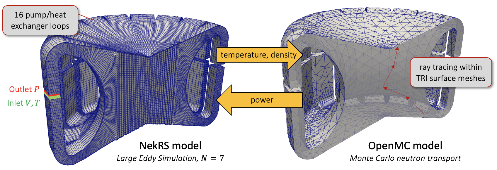
Figure 1: Volume slices through the NekRS and OpenMC domains

As this tutorial is intended primarily to demonstrate on-the-fly geometry skinning, several important features are neglected such as the transport of Delayed Neutron Precursors (DNPs). Future extensions will incorporate material movement in OpenMC driven by velocity (e.g. from a CFD solver such as NekRS), which allows this assumption to be relaxed in the future. For geometric simplicity, radial breeder blankets and axial reflectors are also neglected. The OpenMC model consists of the triangulated surface in Figure 1, with a larger bounding box surrounding it which is set to a vacuum boundary condition.

The nominal operating conditions, as well as the actual conditions used in this tutorial, are summarized in Table 1. In the present tutorial, the reactor is modeled at a 10% flow, 10% power condition (i.e. 300 MWth and 1893 kg/s) to be within an approachable range for Large Eddy Simulation (LES). The NekRS model uses LES at polynomial oder $N=7$ (512 degrees of freedom per element) for 616000 hexahedral elements, or 315 million grid points. Note in Figure 1 that the meshes used by NekRS and OpenMC are very different - the OpenMC domain uses a triangulated mesh, with about 35000 elements.

Table 1: Nominal and simulated operating conditions for the MSFR

Parameter	Nominal Value	Simulated Value
Inlet temperature (K)	898	898
Bulk outlet temperature (K)	998	998
Power (MWth)	3000	300
Mass flowrate (kg/s)	18923	1893

The heat exchanger and pump in each of the 16 legs are replaced by recycling inlet and turbulent outlet boundary conditions for velocity. The recycling inlet boundary condition applies the inlet velocity using the velocity distribution some distance upstream from the outlet boundary, essentially representing the inlet as fully-developed channel flow. The inlet temperature is then set to a uniform value of 898 K. For simplicity, the NekRS model uses an incompressible flow model with constant thermophysical properties from Rouch et al. (2014). A Boussinesq buoyancy term will be added in future work. In the OpenMC model, density feedback is approximated by evaluating a thermophysical property correlation $\rho(T)$ given temperature feedback from NekRS.

OpenMC Model

OpenMC is used to solve for the neutron transport and power distribution. The OpenMC model uses DAGMC for ray tracing within triangular surface meshes in $k$ -eigenvalue mode. The OpenMC model is created using OpenMC's Python API. As shown in Figure 1, the initial OpenMC model consists of a single large volume, enclosed by one large triangulated mesh surface. This geometry will be adaptively updated according to multiphysics feedback.

The OpenMC model is created with the model.py script. The geometry is created from a triangulated volume mesh, exported from Cubit. We create a single material to represent the salt - notice how this contrasts with easlier tutorials for CSG geometries, where we needed to make a unique material for every unique density region. Later, Cardinal will automatically create new materials in memory when we skin the geometry.

import openmc

salt = openmc.Material(name='salt')
salt.set_density('g/cm3', 4.1249)
salt.add_nuclide('Li7', 0.779961, 'ao')
salt.add_nuclide('Li6', 3.89999999999957e-05, 'ao')
salt.add_nuclide('U233', 0.02515, 'ao')
salt.add_element('F', 1.66, 'ao')
salt.add_element('Th', 0.19985, 'ao')
materials = openmc.Materials([salt])
materials.export_to_xml()

dagmc_univ = openmc.DAGMCUniverse(filename="msr.h5m")
geometry = openmc.Geometry(root=dagmc_univ)
geometry.export_to_xml()

settings = openmc.Settings()
lower_left = (-100.0, -100.0, -100.0)
upper_right = (100.0, 100.0, 100.0)
uniform_dist = openmc.stats.Box(lower_left, upper_right)

settings.source = openmc.IndependentSource(space=uniform_dist)

settings.batches = 1500
settings.inactive = 500
settings.particles = 50000

settings.temperature = {'default': 898.0,
                        'method': 'interpolation',
                        'multipole': True,
                        'range': (294.0, 3000.0)}

settings.export_to_xml()

warning

The initial DAGMC model does not contain a graveyard body - so you cannot run this file in a standalone OpenMC run. Cardinal will create a graveyard for you when you have skinning enabled.

You can create these XML files by running

python model.py

or you can simply use the XML files versioned in the directory.

NekRS Model

NekRS is used to solve the incompressible Navier-Stokes equations in non-dimensional form. The NekRS input files needed to solve the incompressible Navier-Stokes equations are:

msfr.re2: NekRS mesh
msfr.par: High-level settings for the solver, boundary condition mappings to sidesets, and the equations to solve
msfr.udf: User-defined C++ functions for on-line postprocessing and model setup
msfr.oudf: User-defined Open Concurrent Compute Abstraction (OCCA) kernels for boundary conditions and source terms
msfr.usr: User-defined Fortran functions; these are used to apply the recycling boundary condition. Long term, eventually all Nek5000 capabilities will be ported to NekRS, and this fortran file would not be necessary.

A detailed description of all of the available parameters, settings, and use cases for these input files is available on the NekRS documentation website. Because the purpose of this analysis is to demonstrate Cardinal's capabilities, only the aspects of NekRS required to understand the present case will be covered.

The mesh is created offline using gmsh, so we simply provide the final mesh on Box. Next, the .par file contains problem setup information. This input solves for pressure, velocity, and temperature. In the nondimensional formulation, the "viscosity" becomes $1/Re$ , where $Re$ is the Reynolds number, while the "thermal conductivity" becomes $1/Pe$ , where $Pe$ is the Peclet number. These nondimensional numbers are used to set various diffusion coefficients in the governing equations with syntax like -4.8e4, which is equivalent in NekRS syntax to $Re=\frac{1}{4.8e4}$ .

We use the high-pass filter in NekRS for the LES, and filter the highest two modes. We set a Reynolds number of $4.8\times10^{4}$ and a Prandtl number of 17.05. We restart this simulation from a previous standalone NekRS run, which used a "frozen" power distribution given in the literature Rouch et al. (2014).

[GENERAL]
  polynomialOrder = 7
  startFrom = restart.fld
  numSteps = 16000
  dt = 2.0e-4
  timeStepper = tombo2
  writeInterval = 2000

  filtering = hpfrt
  filterWeight = 0.1/${dt}
  filterModes = 2

  subCyclingSteps = 2

[PRESSURE]
  residualTol = 1.0e-4

[VELOCITY]
  boundaryTypeMap = inlet, outlet, wall
  residualTol = 1e-6
  density = 1.0
  viscosity = -4.8e4

[TEMPERATURE]
  boundaryTypeMap = inlet, outlet, flux
  rhoCp = 1.0
  conductivity = -818400.0
  residualTol = 1.0e-6

Next, the .udf file is used to set up a heat source GPU kernel which we will use to send OpenMC's heat source from Cardinal into NekRS. As we will show later, this heat source is occupying the first (0-indexed) slot of the scratch space. In the UDF_ExecuteStep, we also do some special copies from some Nek5000 backend data (special usage here to accomplish the recycling boundary conditions) into the 3rd, 4th, and 5th slots of the scratch space (the scratch space is zero-indexed). As shown in the .par file, we will read initial conditions for velocity, pressure, and temperature from a restart file, restart.fld, so we don't need to set any other initial conditions here.

#include <math.h>
#include "udf.hpp"

static occa::kernel mooseHeatSourceKernel;

void userq(nrs_t * nrs, double time, occa::memory o_S, occa::memory o_FS)
{
  // note: when running with Cardinal, Cardinal will allocate the usrwrk
  // array. If running with NekRS standalone (e.g. nrsmpi), you need to
  // replace the usrwrk with some other value or allocate it youself from
  // the udf and populate it with values.
  auto mesh = nrs->cds->mesh[0];
  mooseHeatSourceKernel(mesh->Nelements, 0, nrs->o_usrwrk, o_FS);
}

void UDF_LoadKernels(occa::properties& kernelInfo)
{
   mooseHeatSourceKernel = oudfBuildKernel(kernelInfo, "mooseHeatSource");
}

void UDF_Setup(nrs_t *nrs)
{
  udf.sEqnSource = &userq;
}

void UDF_ExecuteStep(nrs_t *nrs, double time, int tstep)
{
  // call userchk every step for recycle inlet
  nek::ocopyToNek(time, tstep);
  nek::userchk();

 	mesh_t *mesh = nrs->meshV;
  if (tstep == 0)
  {
    double *uin= (double *) nek::scPtr(2);
    nrs->o_usrwrk.copyFrom(uin, mesh->Nelements * mesh->Np * sizeof(dfloat), 2*nrs->fieldOffset*sizeof(dfloat));

    double *vin= (double *) nek::scPtr(3);
    nrs->o_usrwrk.copyFrom(vin, mesh->Nelements * mesh->Np * sizeof(dfloat), 3*nrs->fieldOffset*sizeof(dfloat));

    double *win= (double *) nek::scPtr(4);
    nrs->o_usrwrk.copyFrom(win, mesh->Nelements * mesh->Np * sizeof(dfloat), 4*nrs->fieldOffset*sizeof(dfloat));
  }
}

In the .oudf file, we define boundary conditions and any GPU kernels. We see in velocityDirichletConditions how we are setting the inlet velocities equal to the 3rd, 4th, and 5th slots in the scratch space. The mooseHeatSource is a GPU kernel simply reading from scratch space into the QVOL array (which holds a user-defined volumetric heating).

void velocityDirichletConditions(bcData *bc)
{
  // note: when running with Cardinal, Cardinal will allocate the usrwrk
  // array. If running with NekRS standalone (e.g. nrsmpi), you need to
  // replace the usrwrk with some other value or allocate it youself from
  // the udf and populate it with values.
  bc->u =  bc->usrwrk[bc->idM + 2*bc->fieldOffset];
  bc->v =  bc->usrwrk[bc->idM + 3*bc->fieldOffset];
  bc->w =  bc->usrwrk[bc->idM + 4*bc->fieldOffset];
}

// Stabilized outflow (Dong et al)
void pressureDirichletConditions(bcData *bc)
{
  const dfloat iU0delta = 20.0;
  const dfloat un = bc->u*bc->nx + bc->v*bc->ny + bc->w*bc->nz;
  const dfloat s0 = 0.5 * (1.0 - tanh(un*iU0delta));
  bc->p = -0.5 * (bc->u*bc->u + bc->v*bc->v + bc->w*bc->w) * s0;
}

void scalarDirichletConditions(bcData *bc)
{
  bc->s = 0.0;
}

void scalarNeumannConditions(bcData *bc)
{
  bc->flux = 0.0;
}

@kernel void mooseHeatSource(const dlong Nelements, const dlong offset, @restrict const dfloat * source, @restrict dfloat * QVOL)
{
  for(dlong e=0;e<Nelements;++e;@outer(0)){
    for(int n=0;n<p_Np;++n;@inner(0)){
      const int id = e*p_Np + n;
      QVOL[id] = source[offset + id];
    }
  }
}

Finally, we have a .usr file with Fortran code which accesses from features in Nek5000 which have not yet been fully ported over to NekRS. The code in this file is being used to apply the recycling boundary conditions.

c-----------------------------------------------------------------------
c  nek5000 user-file template
c
c  user specified routines:
c     - uservp  : variable properties
c     - userf   : local acceleration term for fluid
c     - userq   : local source term for scalars
c     - userbc  : boundary conditions
c     - useric  : initial conditions
c     - userchk : general purpose routine for checking errors etc.
c     - userqtl : thermal divergence for lowMach number flows
c     - usrdat  : modify element vertices
c     - usrdat2 : modify mesh coordinates
c     - usrdat3 : general purpose routine for initialization
c
c-----------------------------------------------------------------------
      include "recycle.f"
c-----------------------------------------------------------------------
      subroutine uservp(ix,iy,iz,eg) ! set variable properties
      implicit none
      include 'SIZE'
      include 'TOTAL'
      include 'NEKUSE'

      integer ix,iy,iz,e,eg

      udiff =0.0
      utrans=0.0

      return
      end
c-----------------------------------------------------------------------
      subroutine userf(ix,iy,iz,eg) ! set acceleration term
      implicit none
      include 'SIZE'
      include 'TOTAL'
      include 'NEKUSE'
c
c     Note: this is an acceleration term, NOT a force!
c     Thus, ffx will subsequently be multiplied by rho(x,t).
c
      integer ix,iy,iz,e,eg

      ffx = 0.0
      ffy = 0.0
      ffz = 0.0

      return
      end
c-----------------------------------------------------------------------
      subroutine userq(ix,iy,iz,eg) ! set source term
      implicit none
      include 'SIZE'
      include 'TOTAL'
      include 'NEKUSE'

      integer ix,iy,iz,e,eg

      qvol = 0.0

      return
      end
c-----------------------------------------------------------------------
      subroutine userbc(ix,iy,iz,iside,eg) ! set up boundary conditions
      implicit none
      include 'SIZE'
      include 'TOTAL'
      include 'NEKUSE'

      integer ix,iy,iz,iside,e,eg

      e = gllel(eg)

      ux   = 0.0
      uy   =-1.54261473197
      uz   = 0.0
      temp = 0.0

      return
      end
c-----------------------------------------------------------------------
      subroutine useric(ix,iy,iz,eg) ! set up initial conditions
      implicit none
      include 'SIZE'
      include 'TOTAL'
      include 'NEKUSE'

      integer ix,iy,iz,e,eg

      e = gllel(eg)

      ux   = 0.0
      uy   = 0.0
      uz   = 0.0
      temp = 0.0

      return
      end
c-----------------------------------------------------------------------
      subroutine userchk()
C      implicit none
      include 'SIZE'
      include 'TOTAL'

      real mass_flow_rate

      COMMON /NRSSCPTR/ nrs_scptr(4)
      integer*8         nrs_scptr

      real qt
      common /mauricio/ qt(lx1,ly1,lz1,lelv)

      common /cvelbc/ uin(lx1,ly1,lz1,lelv)
     &              , vin(lx1,ly1,lz1,lelv)
     &              , win(lx1,ly1,lz1,lelv)
     &              , tin(lx1,ly1,lz1,lelt,ldimt)

c recycling boundary conditions
      data ubar / 1.54261473197 /
      data tbar / 0.0 /
      save ubar,tbar

      nxyz = nx1*ny1*nz1
      ntot = nxyz*nelt

      if(istep.eq.0) then
        nrs_scptr(2) = loc(uin(1,1,1,1)) ! pass to udf
        nrs_scptr(3) = loc(vin(1,1,1,1)) ! pass to udf
        nrs_scptr(4) = loc(win(1,1,1,1)) ! pass to udf
      endif

      call set_inflow_fpt(0.0,-0.8,0.0,ubar,tbar) ! for unextruded inlet channels

      call outlet_avgs()

      nrs_scptr(2) = loc(uin(1,1,1,1)) ! pass to udf
      nrs_scptr(3) = loc(vin(1,1,1,1)) ! pass to udf
      nrs_scptr(4) = loc(win(1,1,1,1)) ! pass to udf

      return
      end
c-----------------------------------------------------------------------
      subroutine userqtl ! Set thermal divergence

      call userqtl_scig

      return
      end
c-----------------------------------------------------------------------
      subroutine usrdat()   ! This routine to modify element vertices
      implicit none
      include 'SIZE'
      include 'TOTAL'

      return
      end
c-----------------------------------------------------------------------
      subroutine usrdat2()  ! This routine to modify mesh coordinates
      implicit none
      include 'SIZE'
      include 'TOTAL'

      integer iel, ifc, id_face
      integer i, e, f, n
      real Dhi
      real xx,yy,zz,dr

      do iel=1,nelv
      do ifc=1,2*ndim
        id_face = bc(5,ifc,iel,1)
        if (id_face.eq.1) then        ! surface 1 for inlet
           cbc(ifc,iel,1) = 'v  '
        elseif (id_face.eq.2) then    ! surface 2 for outlet
           cbc(ifc,iel,1) = 'O  '
        elseif (id_face.eq.3) then    ! surface 3 for wall
           cbc(ifc,iel,1) = 'W  '
        endif
      enddo
      enddo

      do i=2,2      !ldimt1
      do e=1,nelt
      do f=1,ldim*2
        cbc(f,e,i)=cbc(f,e,1)
        if(cbc(f,e,1).eq.'W  ') cbc(f,e,i)='t  '
        if(cbc(f,e,1).eq.'v  ') cbc(f,e,i)='t  '
      enddo
      enddo
      enddo

c for boundaryTypeMap in par file
      do iel=1,nelv
      do ifc=1,2*ndim
          boundaryID(ifc,iel) = 0
          boundaryID(ifc,iel) =  bc(5,ifc,iel,1)
          boundaryIDt(ifc,iel) = 0
          boundaryIDt(ifc,iel) =  bc(5,ifc,iel,1)
      enddo
      enddo

      return
      end
c-----------------------------------------------------------------------
      subroutine usrdat3()
      implicit none
      include 'SIZE'
      include 'TOTAL'

      return
      end
C-----------------------------------------------------------------------
      subroutine inlet_avgs(mass_flow_rate)
      include 'SIZE'
      include 'TOTAL'

      real sint2,sarea2
      real tout,touta,TAA,mass_flow_rate

      ntot = lx1*ly1*lz1*nelv

      touta = 0.0
      TAA = 0.0

      do ie=1,nelv
      do ifc=1,2*ldim
        if(cbc(ifc,ie,1).eq.'v  ') then
        call surface_int(sint2,sarea2,vy,ie,ifc)
        TAA= TAA + sarea2
        touta= touta + sint2
        endif
      enddo
      enddo

      touta = glsum(touta,1)
      TAA = glsum(TAA,1)

      mass_flow_rate = touta

      return
      end
c-----------------------------------------------------------------------
c-----------------------------------------------------------------------
      subroutine outlet_avgs()
c      implicit none
      include 'SIZE'
      include 'TOTAL'

      real tout,touta,TAA
      real sint2,sarea2

      ntot = lx1*ly1*lz1*nelv

      touta = 0.0
      TAA = 0.0

      do ie=1,nelv
      do ifc=1,2*ldim
        if(cbc(ifc,ie,1).eq.'O  ') then
        call surface_int(sint2,sarea2,t(1,1,1,1,1),ie,ifc)
        TAA= TAA + sarea2
        touta= touta + sint2
        endif
      enddo
      enddo

      touta = glsum(touta,1)
      TAA = glsum(TAA,1)
      touta = touta/TAA

      return
      end
c-----------------------------------------------------------------------

Multiphysics Coupling

In this section, OpenMC and NekRS are coupled for multiphysics modeling of an MSFR. This section describes all input files.

OpenMC Input Files

The neutron transport is solved using OpenMC. The input file for this portion of the physics is openmc.i. We begin by setting up the mesh mirror, which is the same volumetric mesh used to generate the DAGMC geometry.

[Mesh]
  [mesh]
    type = FileMeshGenerator
    file = msr.e
  []
[]

Next, we set some initial conditions for temperature and density, because we will run OpenMC first.

[ICs]
  [temp]
    type = ConstantIC
    variable = temp
    value = 948.0
  []
  [density]
    type = ConstantIC
    variable = density
    value = '${fparse -0.882*948+4983.6}'
  []
[]

Next, we define a number of auxiliary variables to be used for diagnostic purposes. With the exception of the ParsedAux used to compute a fluid density in terms of temperature, none of the following variables are necessary for coupling, but they will allow us to visualize how data is mapped from OpenMC to the mesh mirror. The CellTemperatureAux and CellDensityAux will display the OpenMC cell temperatures and densities (after volume-averaging from Cardinal).

[AuxVariables]
  [cell_temperature]
    family = MONOMIAL
    order = CONSTANT
  []
  [cell_density]
    family = MONOMIAL
    order = CONSTANT
  []
[]

[AuxKernels]
  [cell_temperature]
    type = CellTemperatureAux
    variable = cell_temperature
  []
  [cell_density]
    type = CellDensityAux
    variable = cell_density
  []
  [density]
    type = ParsedAux
    variable = density
    expression = '-0.882*temp+4983.6'
    coupled_variables = temp
    execute_on = timestep_begin
  []
[]

Next, the [Problem] and [Tallies] blocks define all the parameters related to coupling OpenMC to MOOSE. We will send temperature and density to OpenMC, and extract power using a MeshTally. We set a number of relaxation settings to use Dufek-Gudowski relaxation, which will progressively ramp the number of particles used in the simulation (starting at 5000) so that we selectively apply computational effort only after the thermal-fluid physics are reasonably well converged. Finally, we will be "skinning" the geometry on-the-fly by providing the skinner user object (of type MoabSkinner).

[Problem]
  type = OpenMCCellAverageProblem
  verbose = true

  # this will start each Picard iteration from the fission source from the previous one
  reuse_source = true

  scaling = 100.0

  density_blocks = '1'
  temperature_blocks = '1'
  cell_level = 0

  power = 300.0e6

  relaxation = dufek_gudowski
  first_iteration_particles = 5000

  skinner = moab

  [Tallies]
    [heat_source]
      type = MeshTally
      mesh_template = msr.e
      output = unrelaxed_tally_std_dev
    []
  []
[]

After every Picard iteration, the skinner will group the elements in the mesh according to their temperature and density. For this tutorial, we will group the elements according to temperature by 15 different bins, ranging from a minimum temperature of 800 K up to a maximum temperature of 1150 K. We will then also bin by density, so that we will have a second grouping according to density. Then, we will create a new OpenMC cell for each unique combination of temperature and density, and re-generate the DAGMC mesh surfaces that bound these regions.

Next, we create a NekRS sub-application, and set up transfers of data between OpenMC and NekRS. These transfers will send fluid temperature and density from NekRS up to OpenMC, and a power distribution to NekRS. We will use sub-cycling, and only send data to/from NekRS at those synchronization points, by using the synchronize_in postprocessor transfer.

[MultiApps]
  [nek]
    type = TransientMultiApp
    input_files = 'nek.i'
    sub_cycling = true
    execute_on = timestep_end
  []
[]

[Transfers]
  [temp_to_openmc]
    type = MultiAppGeneralFieldNearestLocationTransfer
    from_multi_app = nek
    variable = temp
    source_variable = temp
  []
  [power_to_nek]
    type = MultiAppGeneralFieldNearestLocationTransfer
    to_multi_app = nek
    source_variable = kappa_fission
    variable = heat_source
  []
  [power_integral_to_nek]
    type = MultiAppPostprocessorTransfer
    to_postprocessor = source_integral
    from_postprocessor = power
    to_multi_app = nek
  []
  [synchronize_in]
    type = MultiAppPostprocessorTransfer
    to_postprocessor = transfer_in
    from_postprocessor = synchronize
    to_multi_app = nek
  []
[]

Finally, we will use a Transient executioner and add a number of postprocessors for diagnostic purposes. We set the "time step" size in OpenMC to be equal to 2000 times the (dimensional) NekRS time step size, so we are essentially running 2000 NekRS time steps for each OpenMC $k$ -eigenvalue solve.

[Postprocessors]
  [power]
    type = ElementIntegralVariablePostprocessor
    variable = kappa_fission
  []
  [k]
    type = KEigenvalue
  []
  [k_std_dev]
    type = KStandardDeviation
  []
  [max_tally_err]
    type = TallyRelativeError
  []
  [max_T]
    type = ElementExtremeValue
    variable = temp
  []
  [avg_T]
    type = ElementAverageValue
    variable = temp
  []
  [max_q]
    type = ElementExtremeValue
    variable = kappa_fission
  []
  [synchronize]
    type = Receiver
    default = 1.0
  []
[]

t_nek = ${fparse 2e-4 * 7.669}

[Executioner]
  type = Transient
  dt = ${fparse 2000 * t_nek}
[]

[Outputs]
  exodus = true
  csv = true
  hide = 'synchronize'
[]

Fluid Input Files

The fluid mass, momentum, and energy transport physics are solved using NekRS. The input file for this portion of the physics is nek.i. We begin by defining a number of file-local constants and by setting up the NekRSMesh mesh mirror. Because we are coupling NekRS via volumetric heating to OepNMC, we need to use a volumetric mesh mirror. The characteristic length chosen for the NekRS files is already 1 m, so we do not need to scale the mesh in any way.

Re = 4.8e4                              # (-)
mu = 0.011266321                        # Pa-s
rho = 4147.3                            # kg/m3

[Mesh]
  type = NekRSMesh
  volume = true
  order = SECOND
[]

The bulk of the NekRS wrapping is specified with NekRSProblem. The NekRS input files are in non-dimensional form, whereas all other coupled applications use dimensional units. The various *_ref and *_0 parameters define the characteristic scales that were used to non-dimensionalize the NekRS input.

[Problem]
  type = NekRSProblem
  casename = 'msfr'
  output = 'temperature'

  synchronization_interval = parent_app

  [Dimensionalize]
    L = 1.0
    U = '${fparse Re * mu / rho}'
    T = '${fparse 625.0 + 273.15}'
    dT = 100.0
    rho = ${rho}
    Cp = 1524.86 # J/kg/K
  []

  normalization_abs_tol = 1e6
  normalization_rel_tol = 1e-3
[]

Then, we simply set up a Transient executioner with the NekTimeStepper.

[Executioner]
  type = Transient
  [TimeStepper]
    type = NekTimeStepper
    min_dt = 1e-10
  []
[]

[Outputs]
  exodus = true
  hide = 'source_integral'
[]

Execution

To run the input files,

mpiexec -np 150 cardinal-opt -i openmc.i

This will produce a number of output files,

openmc_out.e, OpenMC simulation results
openmc_out_nek0.e, NekRS simulation results, mapped to a SECOND order Lagrange basis
moab_skins_*.h5m, OpenMC cell surfaces (in units of centimeters), which can be converted to .vtk format using the mbconvert script
msfr0.f*, NekRS output files

Figure 2 shows the OpenMC power (on a mesh tally), NekRS fluid temperature, and the OpenMC cell temperatures for the last Picard iteration. The black lines delineate the edges of the OpenMC cells, which have been adaptively generated according to the multiphysics feedback.

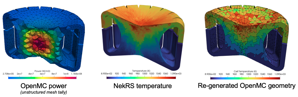
Figure 2: OpenMC power, NekRS fluid temperature, and re-generated OpenMC cells (delinated with black lines) showing the temperature in each cell

References

H. Rouch, O. Geoffroy, P. Rubiolo, A. Laureau, M. Brovchenko, D. Heuer, and E. Merle-Lucotte. Preliminary Thermal-Hydraulic Core Design of the Molten Salt Fast Reactor (MSFR). Annals of Nuclear Energy, 64:449–456, 2014. doi:10.1016/j.anucene.2013.09.012.

@Article{rouch,
    author = "Rouch, H. and Geoffroy, O. and Rubiolo, P. and Laureau, A. and Brovchenko, M. and Heuer, D. and Merle-Lucotte, E.",
    title = "{Preliminary Thermal-Hydraulic Core Design of the Molten Salt Fast Reactor (MSFR)}",
    journal = "Annals of Nuclear Energy",
    volume = "64",
    pages = "449--456",
    year = "2014",
    DOI = "10.1016/j.anucene.2013.09.012"
}

(tutorials/msfr/model.py)

import openmc

salt = openmc.Material(name='salt')
salt.set_density('g/cm3', 4.1249)
salt.add_nuclide('Li7', 0.779961, 'ao')
salt.add_nuclide('Li6', 3.89999999999957e-05, 'ao')
salt.add_nuclide('U233', 0.02515, 'ao')
salt.add_element('F', 1.66, 'ao')
salt.add_element('Th', 0.19985, 'ao')
materials = openmc.Materials([salt])
materials.export_to_xml()

dagmc_univ = openmc.DAGMCUniverse(filename="msr.h5m")
geometry = openmc.Geometry(root=dagmc_univ)
geometry.export_to_xml()

settings = openmc.Settings()
lower_left = (-100.0, -100.0, -100.0)
upper_right = (100.0, 100.0, 100.0)
uniform_dist = openmc.stats.Box(lower_left, upper_right)

settings.source = openmc.IndependentSource(space=uniform_dist)

settings.batches = 1500
settings.inactive = 500
settings.particles = 50000

settings.temperature = {'default': 898.0,
                        'method': 'interpolation',
                        'multipole': True,
                        'range': (294.0, 3000.0)}

settings.export_to_xml()

(tutorials/msfr/msfr.par)

[GENERAL]
  polynomialOrder = 7
  startFrom = restart.fld
  numSteps = 16000
  dt = 2.0e-4
  timeStepper = tombo2
  writeInterval = 2000

  filtering = hpfrt
  filterWeight = 0.1/${dt}
  filterModes = 2

  subCyclingSteps = 2

[PRESSURE]
  residualTol = 1.0e-4

[VELOCITY]
  boundaryTypeMap = inlet, outlet, wall
  residualTol = 1e-6
  density = 1.0
  viscosity = -4.8e4

[TEMPERATURE]
  boundaryTypeMap = inlet, outlet, flux
  rhoCp = 1.0
  conductivity = -818400.0
  residualTol = 1.0e-6

(tutorials/msfr/msfr.udf)

#include <math.h>
#include "udf.hpp"

static occa::kernel mooseHeatSourceKernel;

void userq(nrs_t * nrs, double time, occa::memory o_S, occa::memory o_FS)
{
  // note: when running with Cardinal, Cardinal will allocate the usrwrk
  // array. If running with NekRS standalone (e.g. nrsmpi), you need to
  // replace the usrwrk with some other value or allocate it youself from
  // the udf and populate it with values.
  auto mesh = nrs->cds->mesh[0];
  mooseHeatSourceKernel(mesh->Nelements, 0, nrs->o_usrwrk, o_FS);
}

void UDF_LoadKernels(occa::properties& kernelInfo)
{
   mooseHeatSourceKernel = oudfBuildKernel(kernelInfo, "mooseHeatSource");
}

void UDF_Setup(nrs_t *nrs)
{
  udf.sEqnSource = &userq;
}

void UDF_ExecuteStep(nrs_t *nrs, double time, int tstep)
{
  // call userchk every step for recycle inlet
  nek::ocopyToNek(time, tstep);
  nek::userchk();

 	mesh_t *mesh = nrs->meshV;
  if (tstep == 0)
  {
    double *uin= (double *) nek::scPtr(2);
    nrs->o_usrwrk.copyFrom(uin, mesh->Nelements * mesh->Np * sizeof(dfloat), 2*nrs->fieldOffset*sizeof(dfloat));

    double *vin= (double *) nek::scPtr(3);
    nrs->o_usrwrk.copyFrom(vin, mesh->Nelements * mesh->Np * sizeof(dfloat), 3*nrs->fieldOffset*sizeof(dfloat));

    double *win= (double *) nek::scPtr(4);
    nrs->o_usrwrk.copyFrom(win, mesh->Nelements * mesh->Np * sizeof(dfloat), 4*nrs->fieldOffset*sizeof(dfloat));
  }
}

(tutorials/msfr/msfr.oudf)

void velocityDirichletConditions(bcData *bc)
{
  // note: when running with Cardinal, Cardinal will allocate the usrwrk
  // array. If running with NekRS standalone (e.g. nrsmpi), you need to
  // replace the usrwrk with some other value or allocate it youself from
  // the udf and populate it with values.
  bc->u =  bc->usrwrk[bc->idM + 2*bc->fieldOffset];
  bc->v =  bc->usrwrk[bc->idM + 3*bc->fieldOffset];
  bc->w =  bc->usrwrk[bc->idM + 4*bc->fieldOffset];
}

// Stabilized outflow (Dong et al)
void pressureDirichletConditions(bcData *bc)
{
  const dfloat iU0delta = 20.0;
  const dfloat un = bc->u*bc->nx + bc->v*bc->ny + bc->w*bc->nz;
  const dfloat s0 = 0.5 * (1.0 - tanh(un*iU0delta));
  bc->p = -0.5 * (bc->u*bc->u + bc->v*bc->v + bc->w*bc->w) * s0;
}

void scalarDirichletConditions(bcData *bc)
{
  bc->s = 0.0;
}

void scalarNeumannConditions(bcData *bc)
{
  bc->flux = 0.0;
}

@kernel void mooseHeatSource(const dlong Nelements, const dlong offset, @restrict const dfloat * source, @restrict dfloat * QVOL)
{
  for(dlong e=0;e<Nelements;++e;@outer(0)){
    for(int n=0;n<p_Np;++n;@inner(0)){
      const int id = e*p_Np + n;
      QVOL[id] = source[offset + id];
    }
  }
}

(tutorials/msfr/msfr.usr)

c-----------------------------------------------------------------------
c  nek5000 user-file template
c
c  user specified routines:
c     - uservp  : variable properties
c     - userf   : local acceleration term for fluid
c     - userq   : local source term for scalars
c     - userbc  : boundary conditions
c     - useric  : initial conditions
c     - userchk : general purpose routine for checking errors etc.
c     - userqtl : thermal divergence for lowMach number flows
c     - usrdat  : modify element vertices
c     - usrdat2 : modify mesh coordinates
c     - usrdat3 : general purpose routine for initialization
c
c-----------------------------------------------------------------------
      include "recycle.f"
c-----------------------------------------------------------------------
      subroutine uservp(ix,iy,iz,eg) ! set variable properties
      implicit none
      include 'SIZE'
      include 'TOTAL'
      include 'NEKUSE'

      integer ix,iy,iz,e,eg

      udiff =0.0
      utrans=0.0

      return
      end
c-----------------------------------------------------------------------
      subroutine userf(ix,iy,iz,eg) ! set acceleration term
      implicit none
      include 'SIZE'
      include 'TOTAL'
      include 'NEKUSE'
c
c     Note: this is an acceleration term, NOT a force!
c     Thus, ffx will subsequently be multiplied by rho(x,t).
c
      integer ix,iy,iz,e,eg

      ffx = 0.0
      ffy = 0.0
      ffz = 0.0

      return
      end
c-----------------------------------------------------------------------
      subroutine userq(ix,iy,iz,eg) ! set source term
      implicit none
      include 'SIZE'
      include 'TOTAL'
      include 'NEKUSE'

      integer ix,iy,iz,e,eg

      qvol = 0.0

      return
      end
c-----------------------------------------------------------------------
      subroutine userbc(ix,iy,iz,iside,eg) ! set up boundary conditions
      implicit none
      include 'SIZE'
      include 'TOTAL'
      include 'NEKUSE'

      integer ix,iy,iz,iside,e,eg

      e = gllel(eg)

      ux   = 0.0
      uy   =-1.54261473197
      uz   = 0.0
      temp = 0.0

      return
      end
c-----------------------------------------------------------------------
      subroutine useric(ix,iy,iz,eg) ! set up initial conditions
      implicit none
      include 'SIZE'
      include 'TOTAL'
      include 'NEKUSE'

      integer ix,iy,iz,e,eg

      e = gllel(eg)

      ux   = 0.0
      uy   = 0.0
      uz   = 0.0
      temp = 0.0

      return
      end
c-----------------------------------------------------------------------
      subroutine userchk()
C      implicit none
      include 'SIZE'
      include 'TOTAL'

      real mass_flow_rate

      COMMON /NRSSCPTR/ nrs_scptr(4)
      integer*8         nrs_scptr

      real qt
      common /mauricio/ qt(lx1,ly1,lz1,lelv)


      common /cvelbc/ uin(lx1,ly1,lz1,lelv)
     &              , vin(lx1,ly1,lz1,lelv)
     &              , win(lx1,ly1,lz1,lelv)
     &              , tin(lx1,ly1,lz1,lelt,ldimt)

c recycling boundary conditions
      data ubar / 1.54261473197 /
      data tbar / 0.0 /
      save ubar,tbar

      nxyz = nx1*ny1*nz1
      ntot = nxyz*nelt

      if(istep.eq.0) then
        nrs_scptr(2) = loc(uin(1,1,1,1)) ! pass to udf
        nrs_scptr(3) = loc(vin(1,1,1,1)) ! pass to udf
        nrs_scptr(4) = loc(win(1,1,1,1)) ! pass to udf
      endif

      call set_inflow_fpt(0.0,-0.8,0.0,ubar,tbar) ! for unextruded inlet channels

      call outlet_avgs()

      nrs_scptr(2) = loc(uin(1,1,1,1)) ! pass to udf
      nrs_scptr(3) = loc(vin(1,1,1,1)) ! pass to udf
      nrs_scptr(4) = loc(win(1,1,1,1)) ! pass to udf

      return
      end
c-----------------------------------------------------------------------
      subroutine userqtl ! Set thermal divergence

      call userqtl_scig

      return
      end
c-----------------------------------------------------------------------
      subroutine usrdat()   ! This routine to modify element vertices
      implicit none
      include 'SIZE'
      include 'TOTAL'

      return
      end
c-----------------------------------------------------------------------
      subroutine usrdat2()  ! This routine to modify mesh coordinates
      implicit none
      include 'SIZE'
      include 'TOTAL'

      integer iel, ifc, id_face
      integer i, e, f, n
      real Dhi
      real xx,yy,zz,dr

      do iel=1,nelv
      do ifc=1,2*ndim
        id_face = bc(5,ifc,iel,1)
        if (id_face.eq.1) then        ! surface 1 for inlet
           cbc(ifc,iel,1) = 'v  '
        elseif (id_face.eq.2) then    ! surface 2 for outlet
           cbc(ifc,iel,1) = 'O  '
        elseif (id_face.eq.3) then    ! surface 3 for wall
           cbc(ifc,iel,1) = 'W  '
        endif
      enddo
      enddo

      do i=2,2      !ldimt1
      do e=1,nelt
      do f=1,ldim*2
        cbc(f,e,i)=cbc(f,e,1)
        if(cbc(f,e,1).eq.'W  ') cbc(f,e,i)='t  '
        if(cbc(f,e,1).eq.'v  ') cbc(f,e,i)='t  '
      enddo
      enddo
      enddo

c for boundaryTypeMap in par file
      do iel=1,nelv
      do ifc=1,2*ndim
          boundaryID(ifc,iel) = 0
          boundaryID(ifc,iel) =  bc(5,ifc,iel,1)
          boundaryIDt(ifc,iel) = 0
          boundaryIDt(ifc,iel) =  bc(5,ifc,iel,1)
      enddo
      enddo

      return
      end
c-----------------------------------------------------------------------
      subroutine usrdat3()
      implicit none
      include 'SIZE'
      include 'TOTAL'

      return
      end
C-----------------------------------------------------------------------
      subroutine inlet_avgs(mass_flow_rate)
      include 'SIZE'
      include 'TOTAL'

      real sint2,sarea2
      real tout,touta,TAA,mass_flow_rate

      ntot = lx1*ly1*lz1*nelv

      touta = 0.0
      TAA = 0.0

      do ie=1,nelv
      do ifc=1,2*ldim
        if(cbc(ifc,ie,1).eq.'v  ') then
        call surface_int(sint2,sarea2,vy,ie,ifc)
        TAA= TAA + sarea2
        touta= touta + sint2
        endif
      enddo
      enddo

      touta = glsum(touta,1)
      TAA = glsum(TAA,1)

      mass_flow_rate = touta

      return
      end
c-----------------------------------------------------------------------
c-----------------------------------------------------------------------
      subroutine outlet_avgs()
c      implicit none
      include 'SIZE'
      include 'TOTAL'

      real tout,touta,TAA
      real sint2,sarea2

      ntot = lx1*ly1*lz1*nelv

      touta = 0.0
      TAA = 0.0

      do ie=1,nelv
      do ifc=1,2*ldim
        if(cbc(ifc,ie,1).eq.'O  ') then
        call surface_int(sint2,sarea2,t(1,1,1,1,1),ie,ifc)
        TAA= TAA + sarea2
        touta= touta + sint2
        endif
      enddo
      enddo

      touta = glsum(touta,1)
      TAA = glsum(TAA,1)
      touta = touta/TAA

      return
      end
c-----------------------------------------------------------------------

(tutorials/msfr/openmc.i)

[Mesh]
  [mesh]
    type = FileMeshGenerator
    file = msr.e
  []
[]

[ICs]
  [temp]
    type = ConstantIC
    variable = temp
    value = 948.0
  []
  [density]
    type = ConstantIC
    variable = density
    value = ${fparse -0.882*948+4983.6}
  []
[]

[AuxVariables]
  [cell_temperature]
    family = MONOMIAL
    order = CONSTANT
  []
  [cell_density]
    family = MONOMIAL
    order = CONSTANT
  []
[]

[AuxKernels]
  [cell_temperature]
    type = CellTemperatureAux
    variable = cell_temperature
  []
  [cell_density]
    type = CellDensityAux
    variable = cell_density
  []
  [density]
    type = ParsedAux
    variable = density
    expression = '-0.882*temp+4983.6'
    coupled_variables = temp
    execute_on = timestep_begin
  []
[]

[Problem]
  type = OpenMCCellAverageProblem
  verbose = true

  # this will start each Picard iteration from the fission source from the previous one
  reuse_source = true

  scaling = 100.0

  density_blocks = '1'
  temperature_blocks = '1'
  cell_level = 0

  power = 300.0e6

  relaxation = dufek_gudowski
  first_iteration_particles = 5000

  skinner = moab

  [Tallies]
    [heat_source]
      type = MeshTally
      mesh_template = msr.e
      output = unrelaxed_tally_std_dev
    []
  []
[]

nb = 15.0
tmin = 800.0
tmax = 1150.0

[UserObjects]
  [moab]
    type = MoabSkinner
    temperature = temp
    n_temperature_bins = ${nb}
    temperature_min = ${tmin}
    temperature_max = ${tmax}

    density = density
    n_density_bins = ${nb}
    density_min = ${fparse -0.882*tmax+4983.6}
    density_max = ${fparse -0.882*tmin+4983.6}

    build_graveyard = true
    output_skins = true
  []
[]

[MultiApps]
  [nek]
    type = TransientMultiApp
    input_files = 'nek.i'
    sub_cycling = true
    execute_on = timestep_end
  []
[]

[Transfers]
  [temp_to_openmc]
    type = MultiAppGeneralFieldNearestLocationTransfer
    from_multi_app = nek
    variable = temp
    source_variable = temp
  []
  [power_to_nek]
    type = MultiAppGeneralFieldNearestLocationTransfer
    to_multi_app = nek
    source_variable = kappa_fission
    variable = heat_source
  []
  [power_integral_to_nek]
    type = MultiAppPostprocessorTransfer
    to_postprocessor = source_integral
    from_postprocessor = power
    to_multi_app = nek
  []
  [synchronize_in]
    type = MultiAppPostprocessorTransfer
    to_postprocessor = transfer_in
    from_postprocessor = synchronize
    to_multi_app = nek
  []
[]

[Postprocessors]
  [power]
    type = ElementIntegralVariablePostprocessor
    variable = kappa_fission
  []
  [k]
    type = KEigenvalue
  []
  [k_std_dev]
    type = KStandardDeviation
  []
  [max_tally_err]
    type = TallyRelativeError
  []
  [max_T]
    type = ElementExtremeValue
    variable = temp
  []
  [avg_T]
    type = ElementAverageValue
    variable = temp
  []
  [max_q]
    type = ElementExtremeValue
    variable = kappa_fission
  []
  [synchronize]
    type = Receiver
    default = 1.0
  []
[]

t_nek = ${fparse 2e-4 * 7.669}

[Executioner]
  type = Transient
  dt = ${fparse 2000 * t_nek}
[]

[Outputs]
  exodus = true
  csv = true
  hide = 'synchronize'
[]

(tutorials/msfr/openmc.i)

[Mesh]
  [mesh]
    type = FileMeshGenerator
    file = msr.e
  []
[]

[ICs]
  [temp]
    type = ConstantIC
    variable = temp
    value = 948.0
  []
  [density]
    type = ConstantIC
    variable = density
    value = ${fparse -0.882*948+4983.6}
  []
[]

[AuxVariables]
  [cell_temperature]
    family = MONOMIAL
    order = CONSTANT
  []
  [cell_density]
    family = MONOMIAL
    order = CONSTANT
  []
[]

[AuxKernels]
  [cell_temperature]
    type = CellTemperatureAux
    variable = cell_temperature
  []
  [cell_density]
    type = CellDensityAux
    variable = cell_density
  []
  [density]
    type = ParsedAux
    variable = density
    expression = '-0.882*temp+4983.6'
    coupled_variables = temp
    execute_on = timestep_begin
  []
[]

[Problem]
  type = OpenMCCellAverageProblem
  verbose = true

  # this will start each Picard iteration from the fission source from the previous one
  reuse_source = true

  scaling = 100.0

  density_blocks = '1'
  temperature_blocks = '1'
  cell_level = 0

  power = 300.0e6

  relaxation = dufek_gudowski
  first_iteration_particles = 5000

  skinner = moab

  [Tallies]
    [heat_source]
      type = MeshTally
      mesh_template = msr.e
      output = unrelaxed_tally_std_dev
    []
  []
[]

nb = 15.0
tmin = 800.0
tmax = 1150.0

[UserObjects]
  [moab]
    type = MoabSkinner
    temperature = temp
    n_temperature_bins = ${nb}
    temperature_min = ${tmin}
    temperature_max = ${tmax}

    density = density
    n_density_bins = ${nb}
    density_min = ${fparse -0.882*tmax+4983.6}
    density_max = ${fparse -0.882*tmin+4983.6}

    build_graveyard = true
    output_skins = true
  []
[]

[MultiApps]
  [nek]
    type = TransientMultiApp
    input_files = 'nek.i'
    sub_cycling = true
    execute_on = timestep_end
  []
[]

[Transfers]
  [temp_to_openmc]
    type = MultiAppGeneralFieldNearestLocationTransfer
    from_multi_app = nek
    variable = temp
    source_variable = temp
  []
  [power_to_nek]
    type = MultiAppGeneralFieldNearestLocationTransfer
    to_multi_app = nek
    source_variable = kappa_fission
    variable = heat_source
  []
  [power_integral_to_nek]
    type = MultiAppPostprocessorTransfer
    to_postprocessor = source_integral
    from_postprocessor = power
    to_multi_app = nek
  []
  [synchronize_in]
    type = MultiAppPostprocessorTransfer
    to_postprocessor = transfer_in
    from_postprocessor = synchronize
    to_multi_app = nek
  []
[]

[Postprocessors]
  [power]
    type = ElementIntegralVariablePostprocessor
    variable = kappa_fission
  []
  [k]
    type = KEigenvalue
  []
  [k_std_dev]
    type = KStandardDeviation
  []
  [max_tally_err]
    type = TallyRelativeError
  []
  [max_T]
    type = ElementExtremeValue
    variable = temp
  []
  [avg_T]
    type = ElementAverageValue
    variable = temp
  []
  [max_q]
    type = ElementExtremeValue
    variable = kappa_fission
  []
  [synchronize]
    type = Receiver
    default = 1.0
  []
[]

t_nek = ${fparse 2e-4 * 7.669}

[Executioner]
  type = Transient
  dt = ${fparse 2000 * t_nek}
[]

[Outputs]
  exodus = true
  csv = true
  hide = 'synchronize'
[]

(tutorials/msfr/openmc.i)

[Mesh]
  [mesh]
    type = FileMeshGenerator
    file = msr.e
  []
[]

[ICs]
  [temp]
    type = ConstantIC
    variable = temp
    value = 948.0
  []
  [density]
    type = ConstantIC
    variable = density
    value = ${fparse -0.882*948+4983.6}
  []
[]

[AuxVariables]
  [cell_temperature]
    family = MONOMIAL
    order = CONSTANT
  []
  [cell_density]
    family = MONOMIAL
    order = CONSTANT
  []
[]

[AuxKernels]
  [cell_temperature]
    type = CellTemperatureAux
    variable = cell_temperature
  []
  [cell_density]
    type = CellDensityAux
    variable = cell_density
  []
  [density]
    type = ParsedAux
    variable = density
    expression = '-0.882*temp+4983.6'
    coupled_variables = temp
    execute_on = timestep_begin
  []
[]

[Problem]
  type = OpenMCCellAverageProblem
  verbose = true

  # this will start each Picard iteration from the fission source from the previous one
  reuse_source = true

  scaling = 100.0

  density_blocks = '1'
  temperature_blocks = '1'
  cell_level = 0

  power = 300.0e6

  relaxation = dufek_gudowski
  first_iteration_particles = 5000

  skinner = moab

  [Tallies]
    [heat_source]
      type = MeshTally
      mesh_template = msr.e
      output = unrelaxed_tally_std_dev
    []
  []
[]

nb = 15.0
tmin = 800.0
tmax = 1150.0

[UserObjects]
  [moab]
    type = MoabSkinner
    temperature = temp
    n_temperature_bins = ${nb}
    temperature_min = ${tmin}
    temperature_max = ${tmax}

    density = density
    n_density_bins = ${nb}
    density_min = ${fparse -0.882*tmax+4983.6}
    density_max = ${fparse -0.882*tmin+4983.6}

    build_graveyard = true
    output_skins = true
  []
[]

[MultiApps]
  [nek]
    type = TransientMultiApp
    input_files = 'nek.i'
    sub_cycling = true
    execute_on = timestep_end
  []
[]

[Transfers]
  [temp_to_openmc]
    type = MultiAppGeneralFieldNearestLocationTransfer
    from_multi_app = nek
    variable = temp
    source_variable = temp
  []
  [power_to_nek]
    type = MultiAppGeneralFieldNearestLocationTransfer
    to_multi_app = nek
    source_variable = kappa_fission
    variable = heat_source
  []
  [power_integral_to_nek]
    type = MultiAppPostprocessorTransfer
    to_postprocessor = source_integral
    from_postprocessor = power
    to_multi_app = nek
  []
  [synchronize_in]
    type = MultiAppPostprocessorTransfer
    to_postprocessor = transfer_in
    from_postprocessor = synchronize
    to_multi_app = nek
  []
[]

[Postprocessors]
  [power]
    type = ElementIntegralVariablePostprocessor
    variable = kappa_fission
  []
  [k]
    type = KEigenvalue
  []
  [k_std_dev]
    type = KStandardDeviation
  []
  [max_tally_err]
    type = TallyRelativeError
  []
  [max_T]
    type = ElementExtremeValue
    variable = temp
  []
  [avg_T]
    type = ElementAverageValue
    variable = temp
  []
  [max_q]
    type = ElementExtremeValue
    variable = kappa_fission
  []
  [synchronize]
    type = Receiver
    default = 1.0
  []
[]

t_nek = ${fparse 2e-4 * 7.669}

[Executioner]
  type = Transient
  dt = ${fparse 2000 * t_nek}
[]

[Outputs]
  exodus = true
  csv = true
  hide = 'synchronize'
[]

(tutorials/msfr/openmc.i)

[Mesh]
  [mesh]
    type = FileMeshGenerator
    file = msr.e
  []
[]

[ICs]
  [temp]
    type = ConstantIC
    variable = temp
    value = 948.0
  []
  [density]
    type = ConstantIC
    variable = density
    value = ${fparse -0.882*948+4983.6}
  []
[]

[AuxVariables]
  [cell_temperature]
    family = MONOMIAL
    order = CONSTANT
  []
  [cell_density]
    family = MONOMIAL
    order = CONSTANT
  []
[]

[AuxKernels]
  [cell_temperature]
    type = CellTemperatureAux
    variable = cell_temperature
  []
  [cell_density]
    type = CellDensityAux
    variable = cell_density
  []
  [density]
    type = ParsedAux
    variable = density
    expression = '-0.882*temp+4983.6'
    coupled_variables = temp
    execute_on = timestep_begin
  []
[]

[Problem]
  type = OpenMCCellAverageProblem
  verbose = true

  # this will start each Picard iteration from the fission source from the previous one
  reuse_source = true

  scaling = 100.0

  density_blocks = '1'
  temperature_blocks = '1'
  cell_level = 0

  power = 300.0e6

  relaxation = dufek_gudowski
  first_iteration_particles = 5000

  skinner = moab

  [Tallies]
    [heat_source]
      type = MeshTally
      mesh_template = msr.e
      output = unrelaxed_tally_std_dev
    []
  []
[]

nb = 15.0
tmin = 800.0
tmax = 1150.0

[UserObjects]
  [moab]
    type = MoabSkinner
    temperature = temp
    n_temperature_bins = ${nb}
    temperature_min = ${tmin}
    temperature_max = ${tmax}

    density = density
    n_density_bins = ${nb}
    density_min = ${fparse -0.882*tmax+4983.6}
    density_max = ${fparse -0.882*tmin+4983.6}

    build_graveyard = true
    output_skins = true
  []
[]

[MultiApps]
  [nek]
    type = TransientMultiApp
    input_files = 'nek.i'
    sub_cycling = true
    execute_on = timestep_end
  []
[]

[Transfers]
  [temp_to_openmc]
    type = MultiAppGeneralFieldNearestLocationTransfer
    from_multi_app = nek
    variable = temp
    source_variable = temp
  []
  [power_to_nek]
    type = MultiAppGeneralFieldNearestLocationTransfer
    to_multi_app = nek
    source_variable = kappa_fission
    variable = heat_source
  []
  [power_integral_to_nek]
    type = MultiAppPostprocessorTransfer
    to_postprocessor = source_integral
    from_postprocessor = power
    to_multi_app = nek
  []
  [synchronize_in]
    type = MultiAppPostprocessorTransfer
    to_postprocessor = transfer_in
    from_postprocessor = synchronize
    to_multi_app = nek
  []
[]

[Postprocessors]
  [power]
    type = ElementIntegralVariablePostprocessor
    variable = kappa_fission
  []
  [k]
    type = KEigenvalue
  []
  [k_std_dev]
    type = KStandardDeviation
  []
  [max_tally_err]
    type = TallyRelativeError
  []
  [max_T]
    type = ElementExtremeValue
    variable = temp
  []
  [avg_T]
    type = ElementAverageValue
    variable = temp
  []
  [max_q]
    type = ElementExtremeValue
    variable = kappa_fission
  []
  [synchronize]
    type = Receiver
    default = 1.0
  []
[]

t_nek = ${fparse 2e-4 * 7.669}

[Executioner]
  type = Transient
  dt = ${fparse 2000 * t_nek}
[]

[Outputs]
  exodus = true
  csv = true
  hide = 'synchronize'
[]

(tutorials/msfr/openmc.i)

[Mesh]
  [mesh]
    type = FileMeshGenerator
    file = msr.e
  []
[]

[ICs]
  [temp]
    type = ConstantIC
    variable = temp
    value = 948.0
  []
  [density]
    type = ConstantIC
    variable = density
    value = ${fparse -0.882*948+4983.6}
  []
[]

[AuxVariables]
  [cell_temperature]
    family = MONOMIAL
    order = CONSTANT
  []
  [cell_density]
    family = MONOMIAL
    order = CONSTANT
  []
[]

[AuxKernels]
  [cell_temperature]
    type = CellTemperatureAux
    variable = cell_temperature
  []
  [cell_density]
    type = CellDensityAux
    variable = cell_density
  []
  [density]
    type = ParsedAux
    variable = density
    expression = '-0.882*temp+4983.6'
    coupled_variables = temp
    execute_on = timestep_begin
  []
[]

[Problem]
  type = OpenMCCellAverageProblem
  verbose = true

  # this will start each Picard iteration from the fission source from the previous one
  reuse_source = true

  scaling = 100.0

  density_blocks = '1'
  temperature_blocks = '1'
  cell_level = 0

  power = 300.0e6

  relaxation = dufek_gudowski
  first_iteration_particles = 5000

  skinner = moab

  [Tallies]
    [heat_source]
      type = MeshTally
      mesh_template = msr.e
      output = unrelaxed_tally_std_dev
    []
  []
[]

nb = 15.0
tmin = 800.0
tmax = 1150.0

[UserObjects]
  [moab]
    type = MoabSkinner
    temperature = temp
    n_temperature_bins = ${nb}
    temperature_min = ${tmin}
    temperature_max = ${tmax}

    density = density
    n_density_bins = ${nb}
    density_min = ${fparse -0.882*tmax+4983.6}
    density_max = ${fparse -0.882*tmin+4983.6}

    build_graveyard = true
    output_skins = true
  []
[]

[MultiApps]
  [nek]
    type = TransientMultiApp
    input_files = 'nek.i'
    sub_cycling = true
    execute_on = timestep_end
  []
[]

[Transfers]
  [temp_to_openmc]
    type = MultiAppGeneralFieldNearestLocationTransfer
    from_multi_app = nek
    variable = temp
    source_variable = temp
  []
  [power_to_nek]
    type = MultiAppGeneralFieldNearestLocationTransfer
    to_multi_app = nek
    source_variable = kappa_fission
    variable = heat_source
  []
  [power_integral_to_nek]
    type = MultiAppPostprocessorTransfer
    to_postprocessor = source_integral
    from_postprocessor = power
    to_multi_app = nek
  []
  [synchronize_in]
    type = MultiAppPostprocessorTransfer
    to_postprocessor = transfer_in
    from_postprocessor = synchronize
    to_multi_app = nek
  []
[]

[Postprocessors]
  [power]
    type = ElementIntegralVariablePostprocessor
    variable = kappa_fission
  []
  [k]
    type = KEigenvalue
  []
  [k_std_dev]
    type = KStandardDeviation
  []
  [max_tally_err]
    type = TallyRelativeError
  []
  [max_T]
    type = ElementExtremeValue
    variable = temp
  []
  [avg_T]
    type = ElementAverageValue
    variable = temp
  []
  [max_q]
    type = ElementExtremeValue
    variable = kappa_fission
  []
  [synchronize]
    type = Receiver
    default = 1.0
  []
[]

t_nek = ${fparse 2e-4 * 7.669}

[Executioner]
  type = Transient
  dt = ${fparse 2000 * t_nek}
[]

[Outputs]
  exodus = true
  csv = true
  hide = 'synchronize'
[]

(tutorials/msfr/openmc.i)

[Mesh]
  [mesh]
    type = FileMeshGenerator
    file = msr.e
  []
[]

[ICs]
  [temp]
    type = ConstantIC
    variable = temp
    value = 948.0
  []
  [density]
    type = ConstantIC
    variable = density
    value = ${fparse -0.882*948+4983.6}
  []
[]

[AuxVariables]
  [cell_temperature]
    family = MONOMIAL
    order = CONSTANT
  []
  [cell_density]
    family = MONOMIAL
    order = CONSTANT
  []
[]

[AuxKernels]
  [cell_temperature]
    type = CellTemperatureAux
    variable = cell_temperature
  []
  [cell_density]
    type = CellDensityAux
    variable = cell_density
  []
  [density]
    type = ParsedAux
    variable = density
    expression = '-0.882*temp+4983.6'
    coupled_variables = temp
    execute_on = timestep_begin
  []
[]

[Problem]
  type = OpenMCCellAverageProblem
  verbose = true

  # this will start each Picard iteration from the fission source from the previous one
  reuse_source = true

  scaling = 100.0

  density_blocks = '1'
  temperature_blocks = '1'
  cell_level = 0

  power = 300.0e6

  relaxation = dufek_gudowski
  first_iteration_particles = 5000

  skinner = moab

  [Tallies]
    [heat_source]
      type = MeshTally
      mesh_template = msr.e
      output = unrelaxed_tally_std_dev
    []
  []
[]

nb = 15.0
tmin = 800.0
tmax = 1150.0

[UserObjects]
  [moab]
    type = MoabSkinner
    temperature = temp
    n_temperature_bins = ${nb}
    temperature_min = ${tmin}
    temperature_max = ${tmax}

    density = density
    n_density_bins = ${nb}
    density_min = ${fparse -0.882*tmax+4983.6}
    density_max = ${fparse -0.882*tmin+4983.6}

    build_graveyard = true
    output_skins = true
  []
[]

[MultiApps]
  [nek]
    type = TransientMultiApp
    input_files = 'nek.i'
    sub_cycling = true
    execute_on = timestep_end
  []
[]

[Transfers]
  [temp_to_openmc]
    type = MultiAppGeneralFieldNearestLocationTransfer
    from_multi_app = nek
    variable = temp
    source_variable = temp
  []
  [power_to_nek]
    type = MultiAppGeneralFieldNearestLocationTransfer
    to_multi_app = nek
    source_variable = kappa_fission
    variable = heat_source
  []
  [power_integral_to_nek]
    type = MultiAppPostprocessorTransfer
    to_postprocessor = source_integral
    from_postprocessor = power
    to_multi_app = nek
  []
  [synchronize_in]
    type = MultiAppPostprocessorTransfer
    to_postprocessor = transfer_in
    from_postprocessor = synchronize
    to_multi_app = nek
  []
[]

[Postprocessors]
  [power]
    type = ElementIntegralVariablePostprocessor
    variable = kappa_fission
  []
  [k]
    type = KEigenvalue
  []
  [k_std_dev]
    type = KStandardDeviation
  []
  [max_tally_err]
    type = TallyRelativeError
  []
  [max_T]
    type = ElementExtremeValue
    variable = temp
  []
  [avg_T]
    type = ElementAverageValue
    variable = temp
  []
  [max_q]
    type = ElementExtremeValue
    variable = kappa_fission
  []
  [synchronize]
    type = Receiver
    default = 1.0
  []
[]

t_nek = ${fparse 2e-4 * 7.669}

[Executioner]
  type = Transient
  dt = ${fparse 2000 * t_nek}
[]

[Outputs]
  exodus = true
  csv = true
  hide = 'synchronize'
[]

(tutorials/msfr/nek.i)

Re = 4.8e4                              # (-)
mu = 0.011266321                        # Pa-s
rho = 4147.3                            # kg/m3

[Mesh]
  type = NekRSMesh
  volume = true
  order = SECOND
[]

[Problem]
  type = NekRSProblem
  casename = 'msfr'
  output = 'temperature'

  synchronization_interval = parent_app

  [Dimensionalize]
    L = 1.0
    U = ${fparse Re * mu / rho}
    T = ${fparse 625.0 + 273.15}
    dT = 100.0
    rho = ${rho}
    Cp = 1524.86 # J/kg/K
  []

  normalization_abs_tol = 1e6
  normalization_rel_tol = 1e-3
[]

[Executioner]
  type = Transient
  [TimeStepper]
    type = NekTimeStepper
    min_dt = 1e-10
  []
[]

[Outputs]
  exodus = true
  hide = 'source_integral'
[]

(tutorials/msfr/nek.i)

Re = 4.8e4                              # (-)
mu = 0.011266321                        # Pa-s
rho = 4147.3                            # kg/m3

[Mesh]
  type = NekRSMesh
  volume = true
  order = SECOND
[]

[Problem]
  type = NekRSProblem
  casename = 'msfr'
  output = 'temperature'

  synchronization_interval = parent_app

  [Dimensionalize]
    L = 1.0
    U = ${fparse Re * mu / rho}
    T = ${fparse 625.0 + 273.15}
    dT = 100.0
    rho = ${rho}
    Cp = 1524.86 # J/kg/K
  []

  normalization_abs_tol = 1e6
  normalization_rel_tol = 1e-3
[]

[Executioner]
  type = Transient
  [TimeStepper]
    type = NekTimeStepper
    min_dt = 1e-10
  []
[]

[Outputs]
  exodus = true
  hide = 'source_integral'
[]

(tutorials/msfr/nek.i)

Re = 4.8e4                              # (-)
mu = 0.011266321                        # Pa-s
rho = 4147.3                            # kg/m3

[Mesh]
  type = NekRSMesh
  volume = true
  order = SECOND
[]

[Problem]
  type = NekRSProblem
  casename = 'msfr'
  output = 'temperature'

  synchronization_interval = parent_app

  [Dimensionalize]
    L = 1.0
    U = ${fparse Re * mu / rho}
    T = ${fparse 625.0 + 273.15}
    dT = 100.0
    rho = ${rho}
    Cp = 1524.86 # J/kg/K
  []

  normalization_abs_tol = 1e6
  normalization_rel_tol = 1e-3
[]

[Executioner]
  type = Transient
  [TimeStepper]
    type = NekTimeStepper
    min_dt = 1e-10
  []
[]

[Outputs]
  exodus = true
  hide = 'source_integral'
[]

Geometry and Computational Model
Multiphysics Coupling
Execution
References