Conjugate Heat Transfer for Flow Over a Pebble
In this tutorial, you will learn how to:
Couple NekRS with MOOSE for CHT
Compute a heat transfer coefficient using NekRS
To access this tutorial,
cd cardinal/tutorials/pebble_cht
Geometry and Computational Model
The domain consists of a single pebble within a rectangular box; the pebble origin is at . Figure 1 shows the fluid portion of the domain (the pebble is not shown). The sideset numbering in the fluid domain is:
1: inlet
2: outlet
3: pebble surface
4: side walls
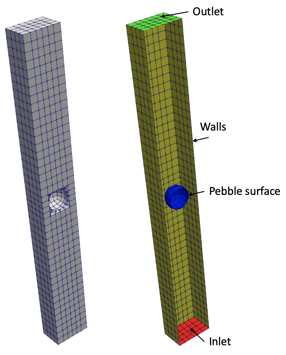
Figure 1: NekRS flow domain. Sidesets in the fluid domain are colored on the right.
NekRS shall solve for laminar flow over this pebble. Details on the problem specifications are given in a previous tutorial. If you have not reviewed this prior tutorial, we highly recommend doing so before proceeding.
The MOOSE heat transfer module shall be used to solve for the solid temperature. NekRS and MOOSE will be coupled through boundary conditions on the pebble surface; NekRS shall compute a pebble surface temperature to be applied as a Dirichlet condition to MOOSE, while MOOSE shall compute a pebble surface heat flux to be applied as a Neumann condition in NekRS.
CHT Coupling
In this example, the overall calculation workflow is as follows:
Run MOOSE heat conduction with a given surface temperature distribution from NekRS.
Send heat flux to NekRS as a boundary condition.
Run NekRS with a given surface heat flux distribution from MOOSE.
Send surface temperature to MOOSE as a boundary condition.
The above sequence is repeated until convergence.
Fluid Input Files
NekRS is used to solve the incompressible Navier-Stokes equations. We already created the input files for NekRS in the NekRS introduction tutorial. If you have not reviewed this tutorial, please be sure to do so before proceeding. We will only describe the aspects of our NekRS setup which differ from this previous tutorial. The .par, .udf, and .usr files are identical from the prior tutorial.
For conjugate heat transfer coupling to MOOSE, we only need to change one line in the NekRS .oudf file to apply a heat flux boundary condition from MOOSE. In the scalarNeumannConditions function, we simply need to set
bc->flux = bc->usrwrk[bc->idM];
We will explain in more detail shortly what this line means. Other than this single change, you are ready to use the same NekRS files to couple to MOOSE.
MOOSE Wrapping
Aside from NekRS's input files, the wrapping of NekRS as a MOOSE application is specified in a "thin" MOOSE-type input file (which we named nek.i for this example).
A mirror of the NekRS mesh is constructed using the NekRSMesh. The boundary parameter indicates the boundaries through which NekRS is coupled to MOOSE.
[Mesh<<<{"href": "../syntax/Mesh/index.html"}>>>]
  type = NekRSMesh

  # This is the boundary we are coupling via conjugate heat transfer to MOOSE
  boundary = '3'
[]Note that pebble.re2 does not appear anywhere in nek.i - the pebble.re2 file is a mesh used directly by NekRS, while NekRSMesh is a mirror of the boundaries in pebble.re2 through which boundary coupling with MOOSE will be performed.
Next, the Problem block describes all objects necessary for the actual physics solve. To replace MOOSE finite element calculations with NekRS spectral element calculations, the NekRSProblem class is used. The casename is used to supply the file name prefix for the NekRS input files.
[Problem<<<{"href": "../syntax/Problem/index.html"}>>>]
  type = NekRSProblem
  casename<<<{"description": "Case name for the NekRS input files; this is <case> in <case>.par, <case>.udf, <case>.oudf, and <case>.re2."}>>> = 'pebble'
  n_usrwrk_slots<<<{"description": "Number of slots to allocate in nrs->usrwrk to hold fields either related to coupling (which will be populated by Cardinal), or other custom usages, such as a distance-to-wall calculation"}>>> = 1

  [FieldTransfers<<<{"href": "../syntax/Problem/FieldTransfers/index.html"}>>>]
    [flux]
      type = NekBoundaryFlux<<<{"description": "Reads/writes boundary flux data between NekRS and MOOSE."}>>>
      direction<<<{"description": "Direction in which to send data"}>>> = to_nek
      usrwrk_slot<<<{"description": "When 'direction = to_nek', the slot(s) in the usrwrk array to write the incoming data; provide one entry for each quantity being passed"}>>> = 0
    []
    [temp]
      type = NekFieldVariable<<<{"description": "Reads/writes volumetric field data between NekRS and MOOSE."}>>>
      direction<<<{"description": "Direction in which to send data"}>>> = from_nek
      field<<<{"description": "NekRS field variable to read/write; defaults to the name of the object"}>>> = temperature
    []
  []
[]The FieldTransfers block then adds the field transfers to represent data passing between nek.i and NekRS's internal data structures. A NekBoundaryFlux is used to write a wall flux into NekRS. This object will automatically create an auxiliary variable named flux and a postprocessor named flux_integral to use for ensuring conservation. Then, the NekFieldVariable is used to fetch temperature from NekRS and write into an auxiliary variable named temp.
Next, a Transient executioner is specified. This is the same executioner used for most transient MOOSE simulations, except now a different time stepper is used - NekTimeStepper. This time stepper simply reads the time step specified in NekRS's .par file. Except for synchronziation points with the MOOSE application(s) to which NekRS is coupled, NekRS controls all of its own time stepping. Note that in this example, NekRS will be run as a sub-application of the heat conduction solve. In this case, the numSteps settings in the .par file are actually ignored, so that the main MOOSE application controls when the simulation terminates.
[Executioner<<<{"href": "../syntax/Executioner/index.html"}>>>]
  type = Transient

  [TimeStepper<<<{"href": "../syntax/Executioner/TimeStepper/index.html"}>>>]
    type = NekTimeStepper
  []
[]An Exodus II output format is specified. It is important to note that this output file only outputs the NekRS solution fields that have been interpolated onto the mesh mirror; the solution over the entire NekRS domain is output with the usual field file format used by standalone NekRS calculations.
[Outputs<<<{"href": "../syntax/Outputs/index.html"}>>>]
  exodus<<<{"description": "Output the results using the default settings for Exodus output."}>>> = true
  csv<<<{"description": "Output the scalar variable and postprocessors to a *.csv file using the default CSV output."}>>> = true
  interval = 10
  hide<<<{"description": "A list of the variables and postprocessors that should NOT be output to the Exodus file (may include Variables, ScalarVariables, and Postprocessor names)."}>>> = 'flux_integral'
[]Solid Input Files
The MOOSE heat transfer module is used to solve for energy conservation in the solid.
First, a local variable, pebble_diameter is used to conveniently be able to repeat data throughout a MOOSE input file. Then, anywhere in the input file that we want to refer to the value 0.03, we can use bash-type syntax like ${pebble_diameter}. Note that these names are completely arbitrary, and simply help to streamline setup for complex MOOSE input files.
You can use similar syntax to do math inside a MOOSE input file. For example, to populate a location in the input file with half the value held by the file-local variable pebble_diameter, you would write ${fparse 0.5 * pebble_diameter}.
The mesh is generated using MOOSE's SphereMeshGenerator. You can either generate this mesh "online" as part of the simulation setup, or we can create it as a separate activity and then load it (just as you can load any Exodus mesh into a MOOSE simulation). We will do the former here, but still show you how you can generate a mesh.
[Mesh<<<{"href": "../syntax/Mesh/index.html"}>>>]
  [sphere]
    type = SphereMeshGenerator<<<{"description": "Generate a 3-D sphere mesh centered on the origin", "href": "../source/meshgenerators/SphereMeshGenerator.html"}>>>
    radius<<<{"description": "Sphere radius"}>>> = '${fparse pebble_diameter / 2.0}'
    nr<<<{"description": "Number of radial elements"}>>> = 3
  []
[]We can run this file in "mesh-only mode" (which will skip all of the solves) to generate an Exodus mesh with
cardinal-opt -i solid.i --mesh-only
which will create a file name solid_in.e which contains the mesh. Note that you do not need to do this! When we run our simulation later, the mesh will already be visible in the output file. This is strictly showing you how you would generate just the mesh from a MOOSE input file. If we open solid_in.e in Paraview, we can see the mesh as shown in Figure 2. The surface of the pebble is sideset 0.
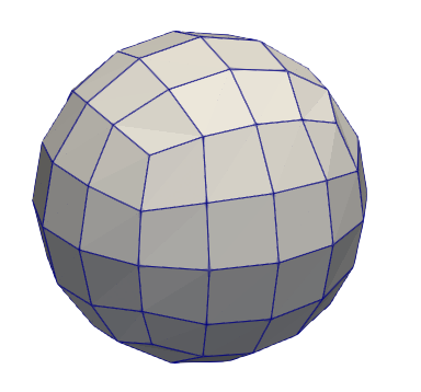
Figure 2: Mesh used for the solid heat conduction.
The heat transfer module will solve for temperature, which is defined as a nonlinear variable.
[Variables<<<{"href": "../syntax/Variables/index.html"}>>>]
  [temp]
  []
[]Next, the governing equation solved by MOOSE is specified with the Kernels block as the HeatConduction kernel plus the BodyForce kernel. On the fluid-solid interface, a MatchedValueBC applies the value of a variable named nek_temp (discussed soon) as a Dirichlet condition. The HeatConduction kernel requires a material property for the thermal conductivity.
[Kernels<<<{"href": "../syntax/Kernels/index.html"}>>>]
  [hc]
    type = HeatConduction<<<{"description": "Diffusive heat conduction term $-\\nabla\\cdot(k\\nabla T)$ of the thermal energy conservation equation", "href": "../source/kernels/HeatConduction.html"}>>>
    variable<<<{"description": "The name of the variable that this residual object operates on"}>>> = temp
  []
  [heat]
    type = BodyForce<<<{"description": "Demonstrates the multiple ways that scalar values can be introduced into kernels, e.g. (controllable) constants, functions, and postprocessors. Implements the weak form $(\\psi_i, -f)$.", "href": "../source/kernels/BodyForce.html"}>>>
    value<<<{"description": "Coefficient to multiply by the body force term"}>>> = 15774023
    variable<<<{"description": "The name of the variable that this residual object operates on"}>>> = temp
  []
[]

[BCs<<<{"href": "../syntax/BCs/index.html"}>>>]
  [match_nek]
    type = MatchedValueBC<<<{"description": "Implements a NodalBC which equates two different Variables' values on a specified boundary.", "href": "../source/bcs/MatchedValueBC.html"}>>>
    variable<<<{"description": "The name of the variable that this residual object operates on"}>>> = temp
    boundary<<<{"description": "The list of boundary IDs from the mesh where this object applies"}>>> = '0'
    v<<<{"description": "The variable whose value we are to match."}>>> = nek_temp
  []
[]

[Materials<<<{"href": "../syntax/Materials/index.html"}>>>]
  [hc]
    type = GenericConstantMaterial<<<{"description": "Declares material properties based on names and values prescribed by input parameters.", "href": "../source/materials/GenericConstantMaterial.html"}>>>
    prop_values<<<{"description": "The values associated with the named properties"}>>> = '${thermal_conductivity}'
    prop_names<<<{"description": "The names of the properties this material will have"}>>> = 'thermal_conductivity'
  []
[]AuxVariables are used to represent field data which passes between different applications. Here, we need to define an auxiliary variable to represent the field data for wall temperature (nek_temp, to be received from NekRS) and the wall heat flux (flux, to be sent to NekRS). A DiffusionFluxAux auxiliary kernel is specified to compute the flux on the fluid_solid_interface boundary. The flux variable must be a monomial field due to the nature of how MOOSE computes material properties.
[AuxVariables<<<{"href": "../syntax/AuxVariables/index.html"}>>>]
  [nek_temp]
  []
  [flux]
    family<<<{"description": "Specifies the family of FE shape functions to use for this variable"}>>> = MONOMIAL
    order<<<{"description": "Specifies the order of the FE shape function to use for this variable (additional orders not listed are allowed)"}>>> = CONSTANT
  []
  [flux_nodal]
  []
[]

[AuxKernels<<<{"href": "../syntax/AuxKernels/index.html"}>>>]
  [flux]
    type = DiffusionFluxAux<<<{"description": "Compute components of flux vector for diffusion problems $(\\vec{J} = -D \\nabla C)$.", "href": "../source/auxkernels/DiffusionFluxAux.html"}>>>
    diffusion_variable<<<{"description": "The name of the variable"}>>> = temp
    component<<<{"description": "The desired component of flux."}>>> = normal
    diffusivity<<<{"description": "The name of the diffusivity material property that will be used in the flux computation."}>>> = thermal_conductivity
    variable<<<{"description": "The name of the variable that this object applies to"}>>> = flux
    boundary<<<{"description": "The list of boundaries (ids or names) from the mesh where this object applies"}>>> = '0'
  []
  [flux_nodal]
    type = ProjectionAux<<<{"description": "Returns the specified variable as an auxiliary variable with a projection of the source variable. If they are the same type, this amounts to a simple copy.", "href": "../source/auxkernels/ProjectionAux.html"}>>>
    variable<<<{"description": "The name of the variable that this object applies to"}>>> = flux_nodal
    v<<<{"description": "Variable to take the value of."}>>> = flux
  []
[]Next, the MultiApps and Transfers blocks describe the interaction between Cardinal and MOOSE. The MOOSE heat transfer module is here run as the main application, with the NekRS wrapping run as the sub-application. We specify that MOOSE will run first on each time step. Allowing sub-cycling means that, if the MOOSE time step is 0.05 seconds, but the NekRS time step set in the .par file is 0.02 seconds, that for every MOOSE time step, NekRS will perform three time steps, of length 0.02, 0.02, and 0.01 seconds to "catch up" to the main application. If sub-cycling is turned off, then the smallest time step among all the various applications is used. This is shown schematically below.
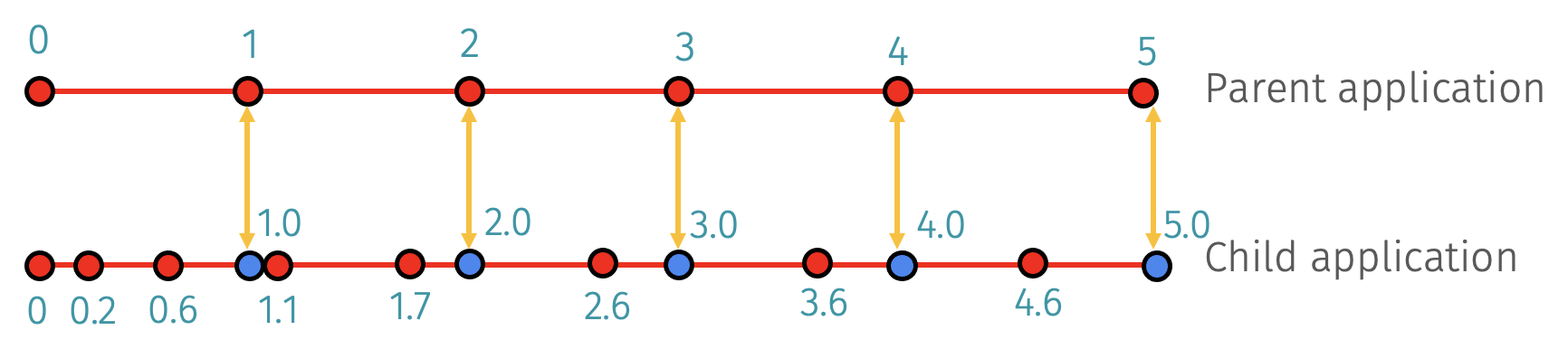
Figure 3: Subcycling in MOOSE will automatically add time steps (blue circles) to the time steps taken by a sub-application to ensure synchronization points. The red circles indicate time steps each application would have taken were it run as a single-physics solve.
Three transfers are required to couple Cardinal and MOOSE; the first is a transfer of surface temperature from Cardinal to MOOSE. The second is a transfer of heat flux from MOOSE to Cardinal. And the third is a transfer of the total integrated heat flux from MOOSE to Cardinal (computed as a postprocessor), which is then used internally by NekRS to re-normalize the heat flux (after interpolation onto NekRS's GLL points).
[MultiApps<<<{"href": "../syntax/MultiApps/index.html"}>>>]
  [nek]
    type = TransientMultiApp<<<{"description": "MultiApp for performing coupled simulations with the parent and sub-application both progressing in time.", "href": "../source/multiapps/TransientMultiApp.html"}>>>
    input_files<<<{"description": "The input file for each App.  If this parameter only contains one input file it will be used for all of the Apps.  When using 'positions_from_file' it is also admissable to provide one input_file per file."}>>> = 'nek.i'
    sub_cycling<<<{"description": "Set to true to allow this MultiApp to take smaller timesteps than the rest of the simulation.  More than one timestep will be performed for each parent application timestep"}>>> = true
  []
[]

[Transfers<<<{"href": "../syntax/Transfers/index.html"}>>>]
  [nek_temp]
    type = MultiAppGeneralFieldNearestLocationTransfer<<<{"description": "Transfers field data at the MultiApp position by finding the value at the nearest neighbor(s) in the origin application.", "href": "../source/transfers/MultiAppGeneralFieldNearestLocationTransfer.html"}>>>
    source_variable<<<{"description": "The variable to transfer from."}>>> = temp
    from_multi_app<<<{"description": "The name of the MultiApp to receive data from"}>>> = nek
    variable<<<{"description": "The auxiliary variable to store the transferred values in."}>>> = nek_temp
  []
  [flux]
    type = MultiAppGeneralFieldNearestLocationTransfer<<<{"description": "Transfers field data at the MultiApp position by finding the value at the nearest neighbor(s) in the origin application.", "href": "../source/transfers/MultiAppGeneralFieldNearestLocationTransfer.html"}>>>
    source_variable<<<{"description": "The variable to transfer from."}>>> = flux_nodal
    to_multi_app<<<{"description": "The name of the MultiApp to transfer the data to"}>>> = nek
    variable<<<{"description": "The auxiliary variable to store the transferred values in."}>>> = flux
  []
  [flux_integral_to_nek]
    type = MultiAppPostprocessorTransfer<<<{"description": "Transfers postprocessor data between the master application and sub-application(s).", "href": "../source/transfers/MultiAppPostprocessorTransfer.html"}>>>
    to_postprocessor<<<{"description": "The name of the Postprocessor in the MultiApp to transfer the value to.  This should most likely be a Reporter Postprocessor."}>>> = flux_integral
    from_postprocessor<<<{"description": "The name of the Postprocessor in the Master to transfer the value from."}>>> = flux_integral
    to_multi_app<<<{"description": "The name of the MultiApp to transfer the data to"}>>> = nek
  []
[]For transfers between two native MOOSE applications, you can ensure conservation of a transferred field using the from_postprocessors_to_be_preserved and to_postprocessors_to_be_preserved options available to any class inheriting from MultiAppConservativeTransfer. However, proper conservation of a field within NekRS (which uses a completely different spatial discretization from MOOSE) requires performing such conservations in NekRS itself. This is why an integral postprocessor must explicitly be passed.
Next, postprocessors are used to compute the integral heat flux as a SideIntegralVariablePostprocessor.
[Postprocessors<<<{"href": "../syntax/Postprocessors/index.html"}>>>]
  [flux_integral]
    type = SideDiffusiveFluxIntegral<<<{"description": "Computes the integral of the diffusive flux over the specified boundary", "href": "../source/postprocessors/SideDiffusiveFluxIntegral.html"}>>>
    diffusivity<<<{"description": "The name of the diffusivity material property that will be used in the flux computation. This must be provided if the variable is of finite element type"}>>> = thermal_conductivity
    variable<<<{"description": "The name of the variable which this postprocessor integrates"}>>> = temp
    boundary<<<{"description": "The list of boundary IDs from the mesh where this object applies"}>>> = '0'
  []
  [max_T]
    type = NodalExtremeValue<<<{"description": "Finds either the min or max elemental value of a variable over the domain.", "href": "../source/postprocessors/NodalExtremeValue.html"}>>>
    variable<<<{"description": "The name of the variable that this postprocessor operates on"}>>> = temp
  []
[]Next, the solution methodology is specified. Although the solid phase only includes time-independent kernels, the heat conduction is run as a transient because NekRS ultimately must be run as a transient (NekRS lacks a steady solver). We choose to omit the time derivative in the solid energy equation because we will reach the converged steady state faster than if the solve had to also ramp up the solid temperature from the initial condition. We will terminate the coupled solve once the relative change in the solid temperature is smaller than the steady_state_tolerance.
[Executioner<<<{"href": "../syntax/Executioner/index.html"}>>>]
  type = Transient

  petsc_options_iname = '-pc_type -pc_hypre_type'
  petsc_options_value = 'hypre boomeramg'

  dt = 5.0
  nl_abs_tol = 1e-8

  steady_state_detection = true
  steady_state_tolerance = 1e-4
[]

[Outputs<<<{"href": "../syntax/Outputs/index.html"}>>>]
  csv<<<{"description": "Output the scalar variable and postprocessors to a *.csv file using the default CSV output."}>>> = true
  exodus<<<{"description": "Output the results using the default settings for Exodus output."}>>> = true
  hide<<<{"description": "A list of the variables and postprocessors that should NOT be output to the Exodus file (may include Variables, ScalarVariables, and Postprocessor names)."}>>> = 'flux_integral flux_nodal'
[]Execution and Postprocessing
To run the conjugate heat transfer model:
mpiexec -np 4 cardinal-opt -i solid.i
which will run with 4 MPI ranks. Both MOOSE and NekRS will be run with 4 processes. When you run Cardinal, a table will be printed out that shows all of the quantities in usrwrk (which is where MOOSE places its heat flux, and is what you used in the .oudf file to apply this boundary condition). This example only exchanges heat flux from MOOSE to NekRS, so the rest of the quantities in this space (called "scratch space") are actually unused. But it is in this table where you can find out what the "slots" in the scratch space represent from MOOSE if you are unsure.
 ===================>     MAPPING FROM MOOSE TO NEKRS      <===================

           Slot:  slice in scratch space holding the data
 MOOSE quantity:  name of the AuxVariable or Postprocessor that gets written into
                  this slot. If 'unused', this means that the space has been
                  allocated, but Cardinal is not otherwise using it for coupling
  How to Access:  C++ code to use in NekRS files; for the .udf instructions,
                  'n' indicates a loop variable over GLL points

-----------------------------------------------------------------------------------------------------------
| Slot | MOOSE quantity |          How to Access (.oudf)          |         How to Access (.udf)          |
-----------------------------------------------------------------------------------------------------------
|    0 | flux           | bc->usrwrk[0 * bc->fieldOffset+bc->idM] | nrs->usrwrk[0 * nrs->fieldOffset + n] |
|    1 | unused         | bc->usrwrk[1 * bc->fieldOffset+bc->idM] | nrs->usrwrk[1 * nrs->fieldOffset + n] |
|    2 | unused         | bc->usrwrk[2 * bc->fieldOffset+bc->idM] | nrs->usrwrk[2 * nrs->fieldOffset + n] |
|    3 | unused         | bc->usrwrk[3 * bc->fieldOffset+bc->idM] | nrs->usrwrk[3 * nrs->fieldOffset + n] |
|    4 | unused         | bc->usrwrk[4 * bc->fieldOffset+bc->idM] | nrs->usrwrk[4 * nrs->fieldOffset + n] |
|    5 | unused         | bc->usrwrk[5 * bc->fieldOffset+bc->idM] | nrs->usrwrk[5 * nrs->fieldOffset + n] |
|    6 | unused         | bc->usrwrk[6 * bc->fieldOffset+bc->idM] | nrs->usrwrk[6 * nrs->fieldOffset + n] |
-----------------------------------------------------------------------------------------------------------
When the simulation has completed, you will have created a number of different output files:
pebble0.f<n>, the NekRS output filessolid_out.e, an Exodus II output file with the solid mesh and solutionsolid_out_nek0.e, an Exodus II output file with the fluid mirror mesh and data that was ultimately transferred in/out of NekRS
First, let's take a look at the two meshes together. Figure 4 shows a slice through the NekRS mesh (with quadrature points shown) and the solid pebble mesh (in yellow). Cardinal does not require conformality between the meshes - by using MOOSE's nearest node transfer, we don't even require overlap between the meshes. Of course there will be some interpolation error when the meshes are not exactly the same, but you can always conduct a mesh refinement study until you are happy with the numerical error in the mapping.
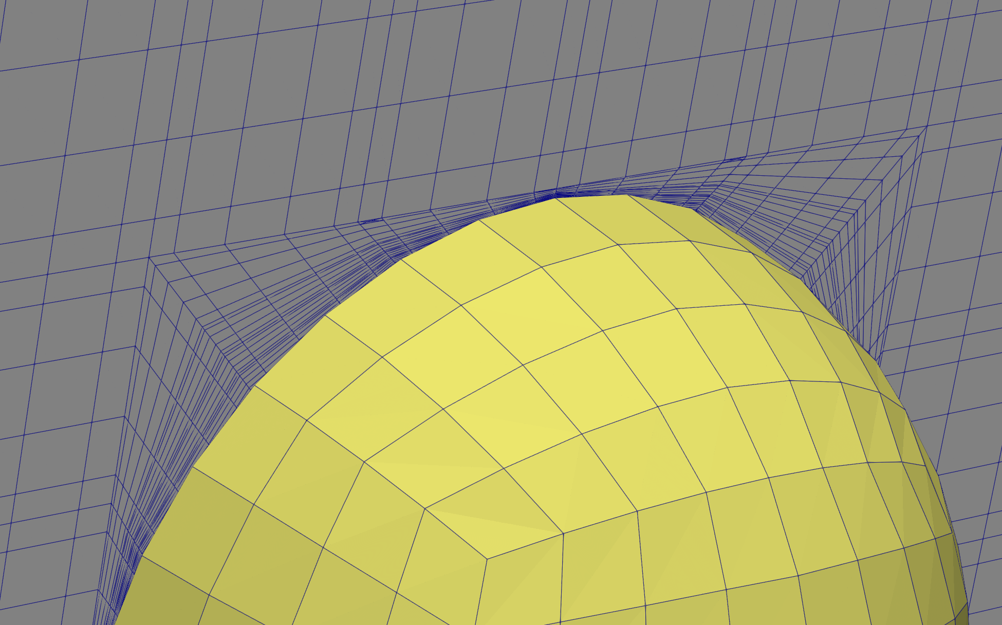
Figure 4: NekRS mesh (gray) and solid mesh (yellow)
Figure 5 shows the fluid temperature (NekRS) and solid temperature (MOOSE). The conjugate heat transfer coupling between the two phases is evident from the continuity in temperature on the pebble surface.
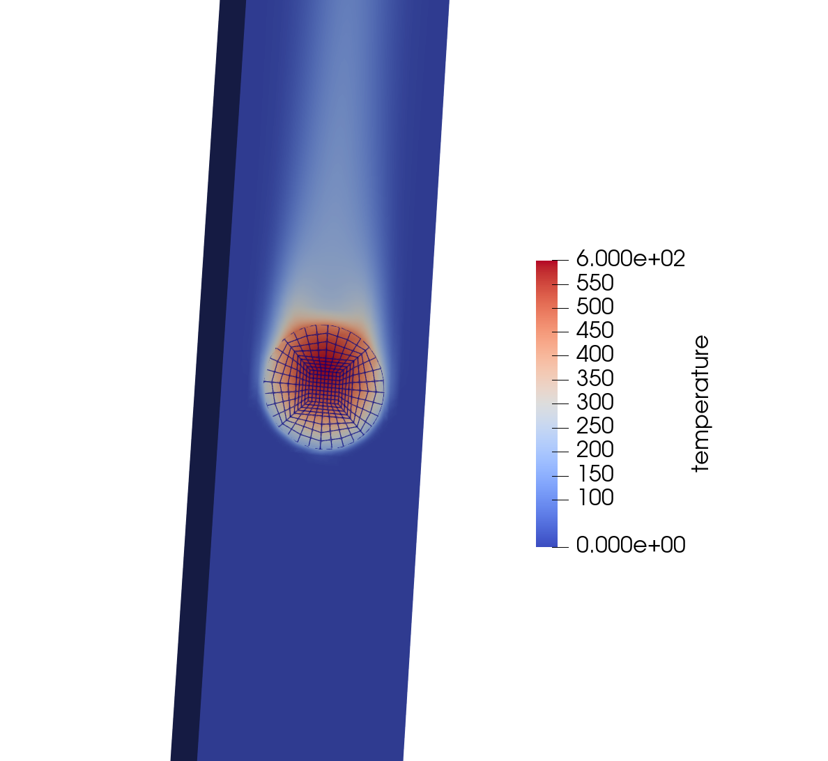
Figure 5: Fluid temperature (NekRS) and solid temperature (MOOSE)
Heat Transfer Coefficients
A heat transfer coefficient is a constitutive model, often generated by a CFD simulation, which can be used in lower-order solvers to _approximately capture the convective heat transfer process_ without needing to resolve boundary layers in those lower-order solvers.
A heat transfer coefficient is defined as
Cardinal contains many postprocessing systems to facilitate the computation of heat transfer coefficients (in addition to other constitutive models). Here, we will add the necessary quantities to the input files and compute a heat transfer coefficient. For reference, we will compare to the following correlation Incropera and Dewitt (2011) for flow over a sphere,
where is based on the sphere diameter and is the Nusselt number, defined as
For , , m, and W/m/K, we should expect that our heat transfer coefficient computed by NekRS is somewhere in the vicinity of 198.45 W/m/K. Of course, in this simple case we already have a published correlation for a Nusselt number - but for more realistic engineering geometries, such correlations may not yet exist!
We need to compute three quantities - , , and . For illustration, we'll compute these as a function of space, and divide up the sphere into 5 axial layers. This is shown conceptually below for the fluid domain (left) and solid domain (right). For each layer, we'll compute (i) the average wall temperature from NekRS, (ii) the average bulk temperature from NekRS, and (iii) the average wall heat flux from MOOSE.
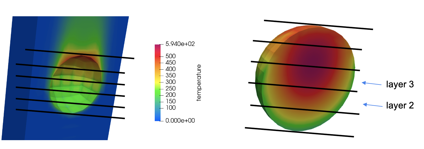
Figure 6: Illustration of the layers to be used for computing the heat transfer coefficient
In the solid file, we add a LayeredSideAverage userobject to evaluate the average surface heat flux in these layers. We then output the results of these userobjects to CSV using SpatialUserObjectVectorPostprocessors and by setting csv = true in the output.
[UserObjects<<<{"href": "../syntax/UserObjects/index.html"}>>>]
  [average_flux_axial]
    type = LayeredSideAverage<<<{"description": "Computes side averages of a variable storing partial sums for the specified number of intervals in a direction (x,y,z).", "href": "../source/userobjects/LayeredSideAverage.html"}>>>
    variable<<<{"description": "The name of the variable that this boundary condition applies to"}>>> = flux
    direction<<<{"description": "The direction of the layers."}>>> = z
    num_layers<<<{"description": "The number of layers."}>>> = 5
    boundary<<<{"description": "The list of boundary IDs from the mesh where this object applies"}>>> = '0'
  []
[]

[VectorPostprocessors<<<{"href": "../syntax/VectorPostprocessors/index.html"}>>>]
  [flux_axial]
    type = SpatialUserObjectVectorPostprocessor<<<{"description": "Outputs the values of a spatial user object in the order of the specified spatial points", "href": "../source/vectorpostprocessors/SpatialUserObjectVectorPostprocessor.html"}>>>
    userobject<<<{"description": "The userobject whose values are to be reported"}>>> = average_flux_axial
  []
[]In the NekRS input file, we add userobjects to compute average wall temperatures and bulk fluid temperatures in axial layers with NekBinnedSideAverage and NekBinnedVolumeAverage objects. We then output the results of these userobjects to CSV using SpatialUserObjectVectorPostprocessors. These objects are actually performing integrations on the actual CFD mesh used by NekRS, so there is no approximation happening from data interpolation to the [Mesh].
[UserObjects<<<{"href": "../syntax/UserObjects/index.html"}>>>]
  [layered_bin]
    type = LayeredBin<<<{"description": "Creates a unique spatial bin for layers in a specified direction", "href": "../source/userobjects/LayeredBin.html"}>>>
    num_layers<<<{"description": "The number of layers between the bounding box of the domain"}>>> = 5
    direction<<<{"description": "The direction of the layers (x, y, or z)"}>>> = z
  []
  [wall_temp]
    type = NekBinnedSideAverage<<<{"description": "Compute the spatially-binned average of a field over a sideset of the NekRS mesh", "href": "../source/userobjects/NekBinnedSideAverage.html"}>>>
    bins<<<{"description": "Userobjects providing a spatial bin given a point"}>>> = 'layered_bin'
    boundary<<<{"description": "Boundary ID(s) over which to compute the bin values"}>>> = '3'
    field<<<{"description": "Field to apply this object to"}>>> = temperature
    map_space_by_qp<<<{"description": "Whether to map the NekRS spatial domain to a bin according to the element centroids (true) or quadrature point locations (false)."}>>> = true
    interval<<<{"description": "Frequency (in number of time steps) with which to execute this user object; user objects can be expensive and not necessary to evaluate on every single time step. NOTE: you probably want to match with 'time_step_interval' in the Output"}>>> = 10
  []
  [bulk_temp]
    type = NekBinnedVolumeAverage<<<{"description": "Compute the spatially-binned volume average of a field over the NekRS mesh", "href": "../source/userobjects/NekBinnedVolumeAverage.html"}>>>
    bins<<<{"description": "Userobjects providing a spatial bin given a point"}>>> = 'layered_bin'
    field<<<{"description": "Field to apply this object to"}>>> = temperature
    map_space_by_qp<<<{"description": "Whether to map the NekRS spatial domain to a bin according to the element centroids (true) or quadrature point locations (false)."}>>> = true
    interval<<<{"description": "Frequency (in number of time steps) with which to execute this user object; user objects can be expensive and not necessary to evaluate on every single time step. NOTE: you probably want to match with 'time_step_interval' in the Output"}>>> = 10
  []
[]

[VectorPostprocessors<<<{"href": "../syntax/VectorPostprocessors/index.html"}>>>]
  [wall]
    type = SpatialUserObjectVectorPostprocessor<<<{"description": "Outputs the values of a spatial user object in the order of the specified spatial points", "href": "../source/vectorpostprocessors/SpatialUserObjectVectorPostprocessor.html"}>>>
    userobject<<<{"description": "The userobject whose values are to be reported"}>>> = wall_temp
  []
  [bulk]
    type = SpatialUserObjectVectorPostprocessor<<<{"description": "Outputs the values of a spatial user object in the order of the specified spatial points", "href": "../source/vectorpostprocessors/SpatialUserObjectVectorPostprocessor.html"}>>>
    userobject<<<{"description": "The userobject whose values are to be reported"}>>> = bulk_temp
  []
[]

[Outputs<<<{"href": "../syntax/Outputs/index.html"}>>>]
  exodus<<<{"description": "Output the results using the default settings for Exodus output."}>>> = true
  csv<<<{"description": "Output the scalar variable and postprocessors to a *.csv file using the default CSV output."}>>> = true
  interval = 10
  hide<<<{"description": "A list of the variables and postprocessors that should NOT be output to the Exodus file (may include Variables, ScalarVariables, and Postprocessor names)."}>>> = 'flux_integral'
[]Now, simply re-run the model:
mpiexec -np 4 cardinal-opt -i solid.i
This will output a number of CSV files. Simply run the htc.py script provided in order to print the average heat transfer coefficient.
import csv
import numpy as np
import glob
import os

Twall = []
Tbulk = []
flux = []

flux_files = glob.glob('solid_out_flux_axial_*')
flux_file = max(flux_files, key=os.path.getctime)
with open(flux_file) as f:
  reader = csv.reader(f, delimiter=',')
  next(f)
  for row in reader:
    flux.append(float(row[0]))

wall_files = glob.glob('solid_out_nek0_wall_*')
wall_file = max(wall_files, key=os.path.getctime)
with open(wall_file) as f:
  reader = csv.reader(f, delimiter=',')
  next(f)
  for row in reader:
    Twall.append(float(row[0]))

bulk_files = glob.glob('solid_out_nek0_bulk_*')
bulk_file = max(bulk_files, key=os.path.getctime)
with open(bulk_file) as f:
  reader = csv.reader(f, delimiter=',')
  next(f)
  for row in reader:
    Tbulk.append(float(row[0]))

h = []
for i in range(len(Twall)):
  h.append(flux[i] / (Twall[i] - Tbulk[i]))

print('The average heat transfer coefficient is (W/m^2K): ', np.mean(h))
Running this script shows that we've computed an average heat transfer coefficient of 197 W/m/K - pretty close to the correlation we are comparing to!
$ python htc.py

The average heat transfer coefficient is (W/m^2K):  197.40833018071388
References
- F.P. Incropera and D.P. Dewitt.
Fundamentals of Heat and Mass Transfer, 7th ed.
John Wiley & Sons, 2011.[BibTeX]