Stochastic Simulations with NekRS

In this tutorial, you will learn how to:

Stochastically perturb multiphysics NekRS simulations for forward Uncertainty Quantification (UQ) using the MOOSE Stochastic Tools Module.

The MOOSE Stochastic Tools Module (STM) is an open-source module in the MOOSE framework for seamlessly integrating massively-parallel UQ, surrogate modeling, and machine learning with MOOSE-based simulations. Here, we will perform a "parameter study" of a conjugate heat transfer coupling of MOOSE heat conduction and NekRS. We will stochastically sample a parameter (the thermal conductivity in the NekRS model) from a distribution $var element = document.getElementById("moose-equation-5d9ffdf0-22ef-42b2-9ae4-f1270ad83a20");katex.render("N", element, {displayMode:false,throwOnError:false});$ times, each time re-running the multiphysics simulation. For each independent run, we will compute a Quantity of Interest (QOI) (maximum NekRS temperature) and evaluate various statistical quantities for that QOI (e.g. mean, standard deviation, confidence intervals).

Cardinal's interface between NekRS and the STM is designed in an infinitely-flexible manner. Any quantity in NekRS which can be modified from the .udf and .oudf files can be stochastically perturbed by MOOSE. In this example, we will just perturb one quantity (thermal conductivity), though you can simultaneously perturb an arbitrary number of parameters. Other notable features include:

You can perturb parameters nested arbitrarily "beneath" the driver stochastic application. We will use this to send a thermal conductivity value from the STM, to a solid heat conduction sub-app, which then passes the value to a NekRS sub-sub app.
You can use a single perturbed value in multiple locations in dependent applications. For example, if you use a multiscale fluid model with NekRS in one part of the domain and the MOOSE Navier-Stokes module in another region of space, you could send a single perturbed value for fluid density to both applications concurrently.

Before reading this tutorial, we recommend reading through Examples 1 through 3 on the STM page to familiarize yourself with the basic syntax for stochastic simulations.

To access this tutorial,


cd cardinal/tutorials/nek_stochastic

Problem Setup

In this problem, we couple a MOOSE solid heat conduction model with a NekRS heat conduction model in two adjacent domains, shown in Figure 1. A uniform heat flux of 1000 W/m $var element = document.getElementById("moose-equation-d6da54d9-6b75-47d6-9c78-2a1b0138d3d6");katex.render("^2", element, {displayMode:false,throwOnError:false});$ is applied on the left face of the MOOSE region, whereas a fixed Dirichlet temperature of 500 K is applied on the right face of the NekRS region. MOOSE and NekRS are coupled via heat flux and temperature on the interface. MOOSE will send a heat flux boundary condition to NekRS, while NekRS will return an interface temperature to MOOSE for use as a Dirichlet condition. All other surfaces are insulated.

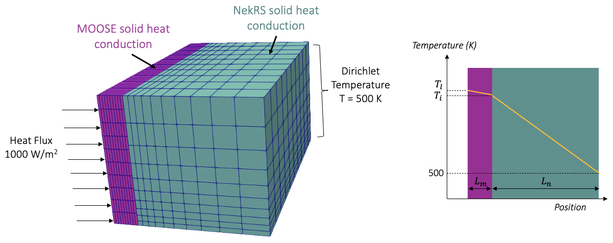
Figure 1: Two-region heat conduction model used for demonstrating stochastic simulations

We choose this problem for demonstration because the steady-state solution has a simple analytic form. The general shape for the temperature distribution is shown as the orange line in the right of Figure 1, where the slopes of the temperature in the two blocks are governed by their respective thermal conductivities. The temperature at the interface, $var element = document.getElementById("moose-equation-d33abf73-0a8d-4a79-9533-e79c90c88d2d");katex.render("T_i", element, {displayMode:false,throwOnError:false});$ , between MOOSE and NekRS is governed by

$(1)var element = document.getElementById("moose-equation-78a26869-4ec1-4e62-b72b-05092ea9d88b");katex.render(" q^{''}=k_n\\frac{T_i-500}{L_{n}}", element, {displayMode:true,throwOnError:false});$

where $var element = document.getElementById("moose-equation-ee6df473-0044-419f-9601-5d5215604665");katex.render("q^{''}", element, {displayMode:false,throwOnError:false});$ is the imposed heat flux on the solid model, $var element = document.getElementById("moose-equation-150b9605-bd35-4d3e-b13f-220b7735169b");katex.render("k_n", element, {displayMode:false,throwOnError:false});$ is the thermal conductivity of the NekRS domain, $var element = document.getElementById("moose-equation-09052423-b156-4cff-8859-d41557cb084f");katex.render("L_n", element, {displayMode:false,throwOnError:false});$ is the width of the NekRS region. Similarly, the temperature at the left face, $var element = document.getElementById("moose-equation-d45ec24d-a7ab-4f4a-aab3-85eb3443249e");katex.render("T_{l}", element, {displayMode:false,throwOnError:false});$ , is governed by

$var element = document.getElementById("moose-equation-725c9456-69a4-4117-94ff-b48e789f9845");katex.render("q^{''}=k_m\\frac{T_l-T_i}{L_{m}}", element, {displayMode:true,throwOnError:false});$

where $var element = document.getElementById("moose-equation-e69a62f1-d8ea-465b-97cf-5d9c8ed1f92f");katex.render("k_m", element, {displayMode:false,throwOnError:false});$ is the thermal conductivity of the MOOSE domain and $var element = document.getElementById("moose-equation-36995e95-da30-4187-a153-68d7509fdb3d");katex.render("L_m", element, {displayMode:false,throwOnError:false});$ is the width of the MOOSE region. We will stochastically perturb $var element = document.getElementById("moose-equation-f8aa0b1e-4b03-4fed-ac09-4933383f460f");katex.render("k_n", element, {displayMode:false,throwOnError:false});$ , the thermal conductivity of the NekRS domain, by sampling it from a normal distribution with mean value of 5.0 and standard deviation of 1.0. For each choice of $var element = document.getElementById("moose-equation-62edb631-a3f4-4969-a45e-3b42ff52d369");katex.render("k_n", element, {displayMode:false,throwOnError:false});$ , we will run this coupled heat transfer model, and predict $var element = document.getElementById("moose-equation-55507bce-ffb2-4243-a7ca-5fdd9c631396");katex.render("T_i", element, {displayMode:false,throwOnError:false});$ as our QOI.

NekRS Model

First, we need to build a mesh for NekRS. We use MOOSE mesh generators to build the rectangular prism with $var element = document.getElementById("moose-equation-7c79fff9-f8af-481a-b2db-fdf8711c5398");katex.render("L_n=1", element, {displayMode:false,throwOnError:false});$ . Because NekRS's sidesets must be numbered contiguously beginning from 1, we need to shift the default sideset IDs created by the GeneratedMeshGenerator.

[Mesh<<<{"href": "../syntax/Mesh/index.html"}>>>]
  [box]
    type = GeneratedMeshGenerator<<<{"description": "Create a line, square, or cube mesh with uniformly spaced or biased elements.", "href": "../source/meshgenerators/GeneratedMeshGenerator.html"}>>>
    dim<<<{"description": "The dimension of the mesh to be generated"}>>> = 3
    nx<<<{"description": "Number of elements in the X direction"}>>> = 10
    ny<<<{"description": "Number of elements in the Y direction"}>>> = 4
    nz<<<{"description": "Number of elements in the Z direction"}>>> = 4
    xmin<<<{"description": "Lower X Coordinate of the generated mesh"}>>> = 0.0
    xmax<<<{"description": "Upper X Coordinate of the generated mesh"}>>> = 1.0
    ymin<<<{"description": "Lower Y Coordinate of the generated mesh"}>>> = 0.0
    ymax<<<{"description": "Upper Y Coordinate of the generated mesh"}>>> = 1.0
    zmin<<<{"description": "Lower Z Coordinate of the generated mesh"}>>> = 0.0
    zmax<<<{"description": "Upper Z Coordinate of the generated mesh"}>>> = 2.0
    bias_x<<<{"description": "The amount by which to grow (or shrink) the cells in the x-direction."}>>> = 1.2
    elem_type<<<{"description": "The type of element from libMesh to generate (default: linear element for requested dimension)"}>>> = HEX20
  []
  [rename]
    type = RenameBoundaryGenerator<<<{"description": "Changes the boundary IDs and/or boundary names for a given set of boundaries defined by either boundary ID or boundary name. The changes are independent of ordering. The merging of boundaries is supported.", "href": "../source/meshgenerators/RenameBoundaryGenerator.html"}>>>
    input<<<{"description": "The mesh we want to modify"}>>> = box
    old_boundary<<<{"description": "Elements with these boundary ID(s)/name(s) will be given the new boundary information specified in 'new_boundary'"}>>> = '0 1 2 3 4 5'
    new_boundary<<<{"description": "The new boundary ID(s)/name(s) to be given by the boundary elements defined in 'old_boundary'."}>>> = '1 2 3 4 5 6'
  []
[]

We can generate an Exodus mesh by running in --mesh-only mode:


cardinal-opt -i channel.i --mesh-only
mv channel_in.e channel.exo

Then, we convert into NekRS's custom .re2 mesh format by running the exo2nek script. Alternatively, you can simply use the channel.re2 file already checked into the repository. The remaining NekRS input files are:

channel.par: High-level settings for the solver, boundary condition mappings to sidesets, and the equations to solve
channel.udf: User-defined C++ functions for on-line postprocessing and model setup
channel.oudf: User-defined OCCA kernels for boundary conditions and source terms

In channel.par, we specify that we want to solve for temperature while disabling the fluid solve by setting solver = none in the [VELOCITY] block. The default initial condition for velocity is a zero value, so this input file is essentially solving for solid heat conduction,

$var element = document.getElementById("moose-equation-01ebf685-6588-4180-a6d7-b86d9f4441a1");katex.render("\\rho C_p\\frac{\\partial T}{\\partial t}-\\nabla\\cdot\\left(k_n\\nabla T\\right)=0", element, {displayMode:true,throwOnError:false});$

where $var element = document.getElementById("moose-equation-f491781b-908a-4843-ba5f-abc70e9eb73a");katex.render("\\rho C_p=50", element, {displayMode:false,throwOnError:false});$ and $var element = document.getElementById("moose-equation-a27391d0-71fd-45bc-b9af-f91897589367");katex.render("k_n", element, {displayMode:false,throwOnError:false});$ will be specified by MOOSE. Normally, all that you need to do to set thermal conductivity in NekRS is to set the conductivity parameter in the [TEMPERATURE] block. Here, we will instead retrieve this value from MOOSE through the .udf.

warning

However, the user must still set conductivity in the .par file because this value is used to initialize the elliptic solvers in NekRS. Do not simply put an arbitrary value here, because an unrealistic value will hamper the convergence of the elliptic solvers for the entire NekRS simulation. In order to initialize the elliptic solvers and preconditioners, we recommend setting the properties in the .par file to their mean values.

[OCCA]
  backend = CPU

[GENERAL]
  stopAt = numSteps
  numSteps = 400
  dt = 1.0
  timeStepper = tombo2
  writeControl = steps
  writeInterval = 500
  polynomialOrder = 5

[VELOCITY]
  solver = none

[PRESSURE]

[TEMPERATURE]
  rhoCp = 50.0
  boundaryTypeMap = insulated, insulated, t, insulated, flux, insulated
  residualTol = 1.0e-6

  # You should set the mean values for any material properties you are
  # perturbing, because these are used to initialize the elliptic solvers
  # for the entire simulation, and you want to use a reasonably representative
  # value here.
  conductivity = 5.0

Next, in the channel.oudf we specify our boundary conditions in the NekRS model – a Dirichlet temperature of 500 on sideset 3 and a heat flux from MOOSE on sideset 5.

void scalarDirichletConditions(bcData * bc)
{
  bc->s = 500.0;
}

void scalarNeumannConditions(bcData * bc)
{
  // note: when running with Cardinal, Cardinal will allocate the usrwrk
  // array. If running with NekRS standalone (e.g. nrsmpi), you need to
  // replace the usrwrk with some other value or allocate it youself from
  // the udf and populate it with values.
  bc->flux = bc->usrwrk[bc->idM];
}

Finally, the channel.udf file contains user-defined functions. Here, we are going to use the udf.properties to apply custom material properties. In the uservp function, we are reading thermal conductivity from the scratch space nrs->usrwrk (to be described in more detail soon). This scratch space is where MOOSE writes any data going into NekRS – which we have used extensively so far to send heat flux, volumetric heating, etc. from MOOSE to NekRS. Now, we will use this same scratch space to fetch a stochastically sampled value for thermal conductivity.

This value is then passed into the thermal conductivity array, slot 0 in o_SProp, by calling the platform->linAlg->fill function. If you wanted to stochastically perturb other quantities, like the fluid viscosity, you would access those in a different way. For a summary of how to access other quantities in NekRS, we will provide a table at the end of this tutorial.

#include "udf.hpp"

void uservp(nrs_t *nrs, double time, occa::memory o_U, occa::memory o_S, occa::memory o_UProp, occa::memory o_SProp)
{
  if (!nrs->usrwrk)
    return;

  dfloat k = nrs->usrwrk[1 * nrs->fieldOffset + 0];

  // apply that value; in nekRS, the 0th slot in o_SProp represents the 'conductivity'
  // field in the par file
  auto mesh = nrs->cds->mesh[0];
  auto o_diff = o_SProp + 0 * nrs->fieldOffset * sizeof(dfloat);
  platform->linAlg->fill(mesh->Nlocal, k, o_diff);
}

void UDF_LoadKernels(occa::properties & kernelInfo)
{
}

void UDF_Setup(nrs_t *nrs)
{
  udf.properties = &uservp;

  auto mesh = nrs->cds->mesh[0];

  int n_gll_points = mesh->Np * mesh->Nelements;
  for (int n = 0; n < n_gll_points; ++n)
    nrs->cds->S[n + 0 * nrs->cds->fieldOffset[0]] = 500.0; // temperature
}

In order to ensure that the most up-to-date stochastic data from MOOSE is used in each scalar and flow solver, we add an extra call to udf.properties in Cardinal each time MOOSE sends new data to NekRS. So, udf.properties is called:

Once before time stepping begins (within nekrs::setup). At this point, nrs->usrwrk does not exist yet, which is why we return without doing anything if nrs->usrwrk is a null pointer (the if (!nrs->usrwrk) line). This means that when the elliptic solvers are initialized, they are using whatever property values are set in the .par file (as already described).
(special to Cardinal) Immediately after MOOSE sends new stochastic data to NekRS
Between each scalar solve and the ensuing flow solve

Steps 1 and 3 already occur in standalone NekRS simulations, so Cardinal is just adding an extra call to ensure consistency.

The last thing we need is the thin wrapper input file which runs NekRS. We start by building a mesh mirror of the NekRS mesh, as a NekRSMesh. We will couple via conjugate heat transfer through boundary 5 in the NekRS domain. Next, we use NekRSProblem to specify that we will replace MOOSE solves with NekRS solves and to add the necessary FieldTransfers to facilitate the conjugate heat transfer boundary conditions. We also add a NekScalarValue scalar transfer, which is how we will send single numbers into NekRS's backend (described shortly). The NekTimeStepper finally will then allow NekRS to control its time stepping, aside from synchronization points imposed by the main app.

[Mesh<<<{"href": "../syntax/Mesh/index.html"}>>>]
  type = NekRSMesh
  boundary = '5'
[]

[Problem<<<{"href": "../syntax/Problem/index.html"}>>>]
  type = NekRSProblem
  casename<<<{"description": "Case name for the NekRS input files; this is <case> in <case>.par, <case>.udf, <case>.oudf, and <case>.re2."}>>> = 'channel'

  [FieldTransfers<<<{"href": "../syntax/Problem/FieldTransfers/index.html"}>>>]
    [flux]
      type = NekBoundaryFlux<<<{"description": "Reads/writes boundary flux data between NekRS and MOOSE."}>>>
      direction<<<{"description": "Direction in which to send data"}>>> = to_nek
      usrwrk_slot<<<{"description": "When 'direction = to_nek', the slot(s) in the usrwrk array to write the incoming data; provide one entry for each quantity being passed"}>>> = 0
    []
    [temperature]
      type = NekFieldVariable<<<{"description": "Reads/writes volumetric field data between NekRS and MOOSE."}>>>
      field<<<{"description": "NekRS field variable to read/write; defaults to the name of the object"}>>> = temperature
      direction<<<{"description": "Direction in which to send data"}>>> = from_nek
    []
  []

  [ScalarTransfers<<<{"href": "../syntax/Problem/ScalarTransfers/index.html"}>>>]
    [k]
      type = NekScalarValue<<<{"description": "Transfers a scalar value into NekRS"}>>>
      direction<<<{"description": "Direction in which to send data"}>>> = to_nek
      usrwrk_slot<<<{"description": "When 'direction = to_nek', the slot in the usrwrk array to write the incoming data"}>>> = 1
      output_postprocessor<<<{"description": "Name of the postprocessor to output the value sent into NekRS"}>>> = k_from_stm
    []
  []
[]

[Executioner<<<{"href": "../syntax/Executioner/index.html"}>>>]
  type = Transient

  [TimeStepper<<<{"href": "../syntax/Executioner/TimeStepper/index.html"}>>>]
    type = NekTimeStepper
  []
[]

[Postprocessors<<<{"href": "../syntax/Postprocessors/index.html"}>>>]
  [max_temp]
    type = NekVolumeExtremeValue<<<{"description": "Extreme value (max/min) of a field over the NekRS mesh", "href": "../source/postprocessors/NekVolumeExtremeValue.html"}>>>
    field<<<{"description": "Field to apply this object to"}>>> = temperature
  []
  [k_from_stm] # this will just print to the screen the value of k received
    type = Receiver<<<{"description": "Reports the value stored in this processor, which is usually filled in by another object. The Receiver does not compute its own value.", "href": "../source/postprocessors/Receiver.html"}>>>
  []
  [expect_max_T]
    type = ParsedPostprocessor<<<{"description": "Computes a parsed expression with post-processors", "href": "../source/postprocessors/ParsedPostprocessor.html"}>>>
    function = '1000.0 / k_from_stm + 500.0'
    pp_names<<<{"description": "Post-processors arguments"}>>> = k_from_stm
  []
[]

[Outputs<<<{"href": "../syntax/Outputs/index.html"}>>>]
  csv<<<{"description": "Output the scalar variable and postprocessors to a *.csv file using the default CSV output."}>>> = true
  hide<<<{"description": "A list of the variables and postprocessors that should NOT be output to the Exodus file (may include Variables, ScalarVariables, and Postprocessor names)."}>>> = 'flux_integral'
[]

[Controls<<<{"href": "../syntax/Controls/index.html"}>>>]
  [stm]
    type = SamplerReceiver<<<{"description": "Control for receiving data from a Sampler via SamplerParameterTransfer.", "href": "../source/controls/SamplerReceiver.html"}>>>
  []
[]

Then, we define a number of postprocessors. The max_temp postprocessor will be our QOI evaluating $var element = document.getElementById("moose-equation-5dffeadc-f46b-4c7b-9093-f07275e7fe6d");katex.render("T_i", element, {displayMode:false,throwOnError:false});$ which will get passed upwards in the multiapp hierarchy. The k_from_stem Receiver postprocessor will be written by our NekScalarValue object for convenience to display the value held by the NekScalarValue transfer to the console so that we can easily see each random value for $var element = document.getElementById("moose-equation-5ea3fcca-44b8-4eed-ac7d-dfb2a96db68b");katex.render("k_n", element, {displayMode:false,throwOnError:false});$ getting received. For sanity check, we also add expect_max_T to compute the analytic value for $var element = document.getElementById("moose-equation-68db1d04-d350-43a0-b8d0-506b986e1f12");katex.render("T_i", element, {displayMode:false,throwOnError:false});$ according to Eq. (1).

[Mesh<<<{"href": "../syntax/Mesh/index.html"}>>>]
  type = NekRSMesh
  boundary = '5'
[]

[Problem<<<{"href": "../syntax/Problem/index.html"}>>>]
  type = NekRSProblem
  casename<<<{"description": "Case name for the NekRS input files; this is <case> in <case>.par, <case>.udf, <case>.oudf, and <case>.re2."}>>> = 'channel'

  [FieldTransfers<<<{"href": "../syntax/Problem/FieldTransfers/index.html"}>>>]
    [flux]
      type = NekBoundaryFlux<<<{"description": "Reads/writes boundary flux data between NekRS and MOOSE."}>>>
      direction<<<{"description": "Direction in which to send data"}>>> = to_nek
      usrwrk_slot<<<{"description": "When 'direction = to_nek', the slot(s) in the usrwrk array to write the incoming data; provide one entry for each quantity being passed"}>>> = 0
    []
    [temperature]
      type = NekFieldVariable<<<{"description": "Reads/writes volumetric field data between NekRS and MOOSE."}>>>
      field<<<{"description": "NekRS field variable to read/write; defaults to the name of the object"}>>> = temperature
      direction<<<{"description": "Direction in which to send data"}>>> = from_nek
    []
  []

  [ScalarTransfers<<<{"href": "../syntax/Problem/ScalarTransfers/index.html"}>>>]
    [k]
      type = NekScalarValue<<<{"description": "Transfers a scalar value into NekRS"}>>>
      direction<<<{"description": "Direction in which to send data"}>>> = to_nek
      usrwrk_slot<<<{"description": "When 'direction = to_nek', the slot in the usrwrk array to write the incoming data"}>>> = 1
      output_postprocessor<<<{"description": "Name of the postprocessor to output the value sent into NekRS"}>>> = k_from_stm
    []
  []
[]

[Executioner<<<{"href": "../syntax/Executioner/index.html"}>>>]
  type = Transient

  [TimeStepper<<<{"href": "../syntax/Executioner/TimeStepper/index.html"}>>>]
    type = NekTimeStepper
  []
[]

[Postprocessors<<<{"href": "../syntax/Postprocessors/index.html"}>>>]
  [max_temp]
    type = NekVolumeExtremeValue<<<{"description": "Extreme value (max/min) of a field over the NekRS mesh", "href": "../source/postprocessors/NekVolumeExtremeValue.html"}>>>
    field<<<{"description": "Field to apply this object to"}>>> = temperature
  []
  [k_from_stm] # this will just print to the screen the value of k received
    type = Receiver<<<{"description": "Reports the value stored in this processor, which is usually filled in by another object. The Receiver does not compute its own value.", "href": "../source/postprocessors/Receiver.html"}>>>
  []
  [expect_max_T]
    type = ParsedPostprocessor<<<{"description": "Computes a parsed expression with post-processors", "href": "../source/postprocessors/ParsedPostprocessor.html"}>>>
    function = '1000.0 / k_from_stm + 500.0'
    pp_names<<<{"description": "Post-processors arguments"}>>> = k_from_stm
  []
[]

[Outputs<<<{"href": "../syntax/Outputs/index.html"}>>>]
  csv<<<{"description": "Output the scalar variable and postprocessors to a *.csv file using the default CSV output."}>>> = true
  hide<<<{"description": "A list of the variables and postprocessors that should NOT be output to the Exodus file (may include Variables, ScalarVariables, and Postprocessor names)."}>>> = 'flux_integral'
[]

Lastly, we need to have a SamplerReceiver, which will actually facilitate receiving the stochastic data into the NekScalarValue object. Any input file receiving stochastic data just needs to have one of these objects.

[Controls<<<{"href": "../syntax/Controls/index.html"}>>>]
  [stm]
    type = SamplerReceiver<<<{"description": "Control for receiving data from a Sampler via SamplerParameterTransfer.", "href": "../source/controls/SamplerReceiver.html"}>>>
  []
[]

Heat Conduction Model

For the MOOSE heat conduction model, we firt set up a mesh and create the nonlinear variables, kernels, and boundary conditions to solve the solid heat conduction equation. The flux auxiliary variable will be used to compute the interface heat flux (which will get sent to NekRS), while the nek_temp auxiliary variable will be a receiver for interface temperature from NekRS. NekRS must run using a transient executioner, so we will use the steady_state_detection feature here to ensure that each NekRS simulation has reached the pseudo-steady state.

[Mesh<<<{"href": "../syntax/Mesh/index.html"}>>>]
  [box]
    type = GeneratedMeshGenerator<<<{"description": "Create a line, square, or cube mesh with uniformly spaced or biased elements.", "href": "../source/meshgenerators/GeneratedMeshGenerator.html"}>>>
    dim<<<{"description": "The dimension of the mesh to be generated"}>>> = 3
    nx<<<{"description": "Number of elements in the X direction"}>>> = 10
    ny<<<{"description": "Number of elements in the Y direction"}>>> = 10
    nz<<<{"description": "Number of elements in the Z direction"}>>> = 10
    xmin<<<{"description": "Lower X Coordinate of the generated mesh"}>>> = -0.2
    xmax<<<{"description": "Upper X Coordinate of the generated mesh"}>>> = 0.0
    ymin<<<{"description": "Lower Y Coordinate of the generated mesh"}>>> = 0.0
    ymax<<<{"description": "Upper Y Coordinate of the generated mesh"}>>> = 1.0
    zmin<<<{"description": "Lower Z Coordinate of the generated mesh"}>>> = 0.0
    zmax<<<{"description": "Upper Z Coordinate of the generated mesh"}>>> = 2.0
  []
[]

[Variables<<<{"href": "../syntax/Variables/index.html"}>>>]
  [temperature]
    initial_condition<<<{"description": "Specifies a constant initial condition for this variable"}>>> = 500.0
  []
[]

[Kernels<<<{"href": "../syntax/Kernels/index.html"}>>>]
  [diffusion]
    type = HeatConduction<<<{"description": "Diffusive heat conduction term $-\\nabla\\cdot(k\\nabla T)$ of the thermal energy conservation equation", "href": "../source/kernels/HeatConduction.html"}>>>
    variable<<<{"description": "The name of the variable that this residual object operates on"}>>> = temperature
    diffusion_coefficient<<<{"description": "Property name of the diffusion coefficient"}>>> = thermal_conductivity
  []
[]

[BCs<<<{"href": "../syntax/BCs/index.html"}>>>]
  [left]
    type = NeumannBC<<<{"description": "Imposes the integrated boundary condition $\\frac{\\partial u}{\\partial n}=h$, where $h$ is a constant, controllable value.", "href": "../source/bcs/NeumannBC.html"}>>>
    variable<<<{"description": "The name of the variable that this residual object operates on"}>>> = temperature
    value<<<{"description": "For a Laplacian problem, the value of the gradient dotted with the normals on the boundary."}>>> = 1000.0
    boundary<<<{"description": "The list of boundary IDs from the mesh where this object applies"}>>> = 'left'
  []
  [interface]
    type = MatchedValueBC<<<{"description": "Implements a NodalBC which equates two different Variables' values on a specified boundary.", "href": "../source/bcs/MatchedValueBC.html"}>>>
    variable<<<{"description": "The name of the variable that this residual object operates on"}>>> = temperature
    v<<<{"description": "The variable whose value we are to match."}>>> = nek_temp
    boundary<<<{"description": "The list of boundary IDs from the mesh where this object applies"}>>> = 'right'
  []
[]

[AuxVariables<<<{"href": "../syntax/AuxVariables/index.html"}>>>]
  [flux]
    family<<<{"description": "Specifies the family of FE shape functions to use for this variable"}>>> = MONOMIAL
    order<<<{"description": "Specifies the order of the FE shape function to use for this variable (additional orders not listed are allowed)"}>>> = CONSTANT
  []
  [nek_temp]
    initial_condition<<<{"description": "Specifies a constant initial condition for this variable"}>>> = 500.0
  []
[]

[AuxKernels<<<{"href": "../syntax/AuxKernels/index.html"}>>>]
  [flux]
    type = DiffusionFluxAux<<<{"description": "Compute components of flux vector for diffusion problems $(\\vec{J} = -D \\nabla C)$.", "href": "../source/auxkernels/DiffusionFluxAux.html"}>>>
    variable<<<{"description": "The name of the variable that this object applies to"}>>> = flux
    diffusion_variable<<<{"description": "The name of the variable"}>>> = temperature
    component<<<{"description": "The desired component of flux."}>>> = normal
    diffusivity<<<{"description": "The name of the diffusivity material property that will be used in the flux computation."}>>> = thermal_conductivity
    boundary<<<{"description": "The list of boundaries (ids or names) from the mesh where this object applies"}>>> = 'right'
  []
[]

[Materials<<<{"href": "../syntax/Materials/index.html"}>>>]
  [k]
    type = GenericConstantMaterial<<<{"description": "Declares material properties based on names and values prescribed by input parameters.", "href": "../source/materials/GenericConstantMaterial.html"}>>>
    prop_names<<<{"description": "The names of the properties this material will have"}>>> = 'thermal_conductivity'
    prop_values<<<{"description": "The values associated with the named properties"}>>> = '1.5'
  []
[]

[Postprocessors<<<{"href": "../syntax/Postprocessors/index.html"}>>>]
  [flux_integral]
    type = SideIntegralVariablePostprocessor<<<{"description": "Computes a surface integral of the specified variable", "href": "../source/postprocessors/SideIntegralVariablePostprocessor.html"}>>>
    variable<<<{"description": "The name of the variable which this postprocessor integrates"}>>> = flux
    boundary<<<{"description": "The list of boundary IDs from the mesh where this object applies"}>>> = 'right'
  []
[]

[Executioner<<<{"href": "../syntax/Executioner/index.html"}>>>]
  type = Transient
  dt = 10.0
  nl_abs_tol = 1e-8

  steady_state_detection = true
  steady_state_tolerance = 5e-4
  steady_state_start_time = 30.0
[]

Next, we add NekRS as a sub-app, and define the transfers. The temperature, flux, and flux_integral transfers we have seen many times before – these are transferring data necessary to apply the heat flux and temperature coupled boundary conditions on the interfaces. The MultiAppReporterTransfer is used to fetch the value held by the max_temp postprocessor in the nek.i input file. A Reporter is basically a vector-valued postprocessor which could be used to hold multiple QOIs. In this example, we are just interested in one value.

[MultiApps<<<{"href": "../syntax/MultiApps/index.html"}>>>]
  [nek]
    type = TransientMultiApp<<<{"description": "MultiApp for performing coupled simulations with the parent and sub-application both progressing in time.", "href": "../source/multiapps/TransientMultiApp.html"}>>>
    input_files<<<{"description": "The input file for each App.  If this parameter only contains one input file it will be used for all of the Apps.  When using 'positions_from_file' it is also admissable to provide one input_file per file."}>>> = 'nek.i'
    sub_cycling<<<{"description": "Set to true to allow this MultiApp to take smaller timesteps than the rest of the simulation.  More than one timestep will be performed for each parent application timestep"}>>> = true
    execute_on<<<{"description": "The list of flag(s) indicating when this object should be executed. For a description of each flag, see https://mooseframework.inl.gov/source/interfaces/SetupInterface.html."}>>> = timestep_end
    wait_for_first_app_init<<<{"description": "Create the first sub-application on rank 0, then MPI_Barrier before creating the next N-1 apps (on all ranks). This is only needed if your sub-application needs to perform some setup actions in quiet, without other sub-applications working at the same time."}>>> = true
  []
[]

[Transfers<<<{"href": "../syntax/Transfers/index.html"}>>>]
  [temperature]
    type = MultiAppGeneralFieldNearestLocationTransfer<<<{"description": "Transfers field data at the MultiApp position by finding the value at the nearest neighbor(s) in the origin application.", "href": "../source/transfers/MultiAppGeneralFieldNearestLocationTransfer.html"}>>>
    source_variable<<<{"description": "The variable to transfer from."}>>> = temperature
    from_multi_app<<<{"description": "The name of the MultiApp to receive data from"}>>> = nek
    variable<<<{"description": "The auxiliary variable to store the transferred values in."}>>> = nek_temp
  []
  [flux]
    type = MultiAppGeneralFieldNearestLocationTransfer<<<{"description": "Transfers field data at the MultiApp position by finding the value at the nearest neighbor(s) in the origin application.", "href": "../source/transfers/MultiAppGeneralFieldNearestLocationTransfer.html"}>>>
    source_variable<<<{"description": "The variable to transfer from."}>>> = flux
    to_multi_app<<<{"description": "The name of the MultiApp to transfer the data to"}>>> = nek
    variable<<<{"description": "The auxiliary variable to store the transferred values in."}>>> = flux
    from_boundaries<<<{"description": "The boundary we are transferring from (if not specified, whole domain is used)."}>>> = 'right'
  []
  [flux_integral]
    type = MultiAppPostprocessorTransfer<<<{"description": "Transfers postprocessor data between the master application and sub-application(s).", "href": "../source/transfers/MultiAppPostprocessorTransfer.html"}>>>
    to_postprocessor<<<{"description": "The name of the Postprocessor in the MultiApp to transfer the value to.  This should most likely be a Reporter Postprocessor."}>>> = flux_integral
    from_postprocessor<<<{"description": "The name of the Postprocessor in the Master to transfer the value from."}>>> = flux_integral
    to_multi_app<<<{"description": "The name of the MultiApp to transfer the data to"}>>> = nek
  []
  [get_qoi]
    type = MultiAppReporterTransfer<<<{"description": "Transfers reporter data between two applications.", "href": "../source/transfers/MultiAppReporterTransfer.html"}>>>
    from_multi_app<<<{"description": "The name of the MultiApp to receive data from"}>>> = nek
    from_reporters<<<{"description": "List of the reporter names (object_name/value_name) to transfer the value from."}>>> = 'max_temp/value'
    to_reporters<<<{"description": "List of the reporter names (object_name/value_name) to transfer the value to."}>>> = 'receive/nek_max_T'
  []
[]

[Outputs<<<{"href": "../syntax/Outputs/index.html"}>>>]
  print_linear_residuals<<<{"description": "Enable printing of linear residuals to the screen (Console)"}>>> = false
  hide<<<{"description": "A list of the variables and postprocessors that should NOT be output to the Exodus file (may include Variables, ScalarVariables, and Postprocessor names)."}>>> = 'flux_integral'
[]

Finally, we declare a ConstantReporter to be the receiving point of the data fetched by the get_qoi transfer. Note that we do not need a SamplerReceiver in this input file because the MOOSE heat conduction model itself is not receiving any stochastic inputs - the NekRS thermal conductivity passes straight from the STM to NekRS.

[Reporters<<<{"href": "../syntax/Reporters/index.html"}>>>]
  [receive]
    type = ConstantReporter<<<{"description": "Reporter with constant values to be accessed by other objects, can be modified using transfers.", "href": "../source/reporters/ConstantReporter.html"}>>>
    real_names<<<{"description": "Names for each real value."}>>> = 'nek_max_T'

    # This value doesnt do anything - you just need to have a dummy here
    real_values<<<{"description": "Values for reals."}>>> = 0.0
  []
[]

Stochastic Tools Module

For stochastic simulations, a STM input "drives" the entire simulation as the main app. First, we define random distributions and sampling methods for our random data. Here, we will use a normal distribution for $var element = document.getElementById("moose-equation-8b5f19b9-5953-461f-bf9b-b9eb8182b6e5");katex.render("k_n", element, {displayMode:false,throwOnError:false});$ . We choose a MonteCarlo sampler to randomly sample from this normal distribution. Here, num_rows is the number of independent samples to take.

[StochasticTools<<<{"href": "../syntax/StochasticTools/index.html"}>>>]
[]

[Distributions<<<{"href": "../syntax/Distributions/index.html"}>>>]
  [dist]
    type = Normal<<<{"description": "Normal distribution", "href": "../source/distributions/Normal.html"}>>>
    mean<<<{"description": "Mean (or expectation) of the distribution."}>>> = 5.0
    standard_deviation<<<{"description": "Standard deviation of the distribution "}>>> = 1.0
  []
[]

[Samplers<<<{"href": "../syntax/Samplers/index.html"}>>>]
  [sample]
    type = MonteCarlo<<<{"description": "Monte Carlo Sampler.", "href": "../source/samplers/MonteCarloSampler.html"}>>>
    num_rows<<<{"description": "The number of rows per matrix to generate."}>>> = 3
    distributions<<<{"description": "The distribution names to be sampled, the number of distributions provided defines the number of columns per matrix."}>>> = 'dist'
  []
[]

Next, we add the MOOSE heat conduction model as a SamplerFullSolveMultiApp, which will launch one new physics simulation for each random sample. We next use a SamplerParameterTransfer to send the random numbers from the sample object into the k UserObject in the sub-sub app named nek. In order to fetch the QOI from the nested physics apps, we use a SamplerReporterTransfer to get the $var element = document.getElementById("moose-equation-ffd3abea-ddbf-4e8d-b2e0-f2c2389aa0d7");katex.render("T_i", element, {displayMode:false,throwOnError:false});$ from the sub-app. This will be held by the storage StochasticMatrix. Finally, we use a StatisticsReporter to conduct some statistical analysis on our QOI.

[MultiApps<<<{"href": "../syntax/MultiApps/index.html"}>>>]
  [ht]
    type = SamplerFullSolveMultiApp<<<{"description": "Creates a full-solve type sub-application for each row of each Sampler matrix.", "href": "../source/multiapps/SamplerFullSolveMultiApp.html"}>>>
    input_files<<<{"description": "The input file for each App.  If this parameter only contains one input file it will be used for all of the Apps.  When using 'positions_from_file' it is also admissable to provide one input_file per file."}>>> = ht.i
    sampler<<<{"description": "The Sampler object to utilize for creating MultiApps."}>>> = sample
    mode<<<{"description": "The operation mode, 'normal' creates one sub-application for each row in the Sampler and 'batch-reset' and 'batch-restore' creates N sub-applications, where N is the minimum of 'num_rows' in the Sampler and floor(number of processes / min_procs_per_app). To run the rows in the Sampler, 'batch-reset' will destroy and re-create sub-apps as needed, whereas the 'batch-restore' will backup and restore sub-apps to the initial state prior to execution, without destruction."}>>> = batch-restore
    wait_for_first_app_init<<<{"description": "Create the first sub-application on rank 0, then MPI_Barrier before creating the next N-1 apps (on all ranks). This is only needed if your sub-application needs to perform some setup actions in quiet, without other sub-applications working at the same time."}>>> = true
  []
[]

[Transfers<<<{"href": "../syntax/Transfers/index.html"}>>>]
  [transer_random_inputs_to_nek]
    type = SamplerParameterTransfer<<<{"description": "Copies Sampler data to a SamplerReceiver object.", "href": "../source/transfers/SamplerParameterTransfer.html"}>>>
    to_multi_app<<<{"description": "The name of the MultiApp to transfer the data to"}>>> = ht
    sampler<<<{"description": "A the Sampler object that Transfer is associated.."}>>> = sample

    # you can send data down to arbitrarily-nested sub-apps
    parameters<<<{"description": "A list of parameters (on the sub application) to control with the Sampler data. The order of the parameters listed here should match the order of the items in the Sampler."}>>> = 'nek:Problem/ScalarTransfers/k/value'
  []
  [results]
    type = SamplerReporterTransfer<<<{"description": "Transfers data from Reporters on the sub-application to a StochasticReporter on the main application.", "href": "../source/transfers/SamplerReporterTransfer.html"}>>>
    from_multi_app<<<{"description": "The name of the MultiApp to receive data from"}>>> = ht
    sampler<<<{"description": "A the Sampler object that Transfer is associated.."}>>> = sample
    stochastic_reporter<<<{"description": "The name of the StochasticReporter object to transfer values to."}>>> = storage
    from_reporter<<<{"description": "The name(s) of the Reporter(s) on the sub-app to transfer from."}>>> = 'receive/nek_max_T'
  []
[]

[Reporters<<<{"href": "../syntax/Reporters/index.html"}>>>]
  [storage]
    type = StochasticMatrix<<<{"description": "Tool for extracting Sampler object data and storing data from stochastic simulations.", "href": "../source/reporters/StochasticMatrix.html"}>>>
    sampler<<<{"description": "The sample from which to extract distribution data."}>>> = sample
    parallel_type<<<{"description": "This parameter will determine how the stochastic data is gathered. It is common for outputting purposes that this parameter be set to ROOT, otherwise, many files will be produced showing the values on each processor. However, if there are lot of samples, gathering on root may be memory restrictive."}>>> = ROOT
  []
  [stats]
    type = StatisticsReporter<<<{"description": "Compute statistical values of a given VectorPostprocessor objects and vectors.", "href": "../source/reporters/StatisticsReporter.html"}>>>
    reporters<<<{"description": "List of Reporter values to utilized for statistic computations."}>>> = 'storage/results:receive:nek_max_T'
    compute<<<{"description": "The statistic(s) to compute for each of the supplied vector postprocessors."}>>> = 'mean stddev'
    ci_method<<<{"description": "The method to use for computing confidence level intervals."}>>> = 'percentile'
    ci_levels<<<{"description": "A vector of confidence levels to consider, values must be in (0, 1)."}>>> = '0.05 0.95'
  []
[]

[Outputs<<<{"href": "../syntax/Outputs/index.html"}>>>]
  execute_on<<<{"description": "The list of flag(s) indicating when this object should be executed. For a description of each flag, see https://mooseframework.inl.gov/source/interfaces/SetupInterface.html."}>>> = timestep_end
  [out]
    type = JSON<<<{"description": "Output for Reporter values using JSON format.", "href": "../source/outputs/JSONOutput.html"}>>>
  []
[]

Summary

Figure 2 summarizes the data flow for this stochastic simulation. The only specialization for NekRS is the use of NekScalarValue to receive the data, which the user is then responsible for applying in the NekRS input files as appropriate.

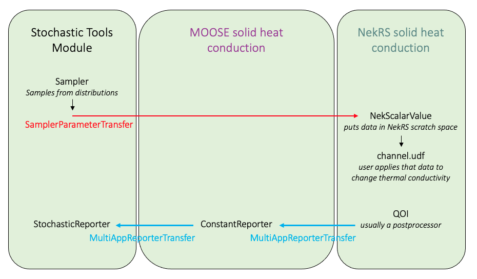
Figure 2: Summary of major data transfers and objects used to accomplish stochastic simulations with NekRS

Execution and Postprocessing

To run the stochastic simulation


mpiexec -np 2 cardinal-opt -i driver.i

When you first run this input file, you will see a table print at the beginning of the NekRS solve which shows:


 -----------------------------------------------------------------------------------------------------------
 | Slot | MOOSE quantity |          How to Access (.oudf)          |         How to Access (.udf)          |
 -----------------------------------------------------------------------------------------------------------
 |    0 | flux           | bc->usrwrk[0 * bc->fieldOffset+bc->idM] | nrs->usrwrk[0 * nrs->fieldOffset + n] |
 |    1 | k              | bc->usrwrk[1 * bc->fieldOffset + 0]     | nrs->usrwrk[1 * nrs->fieldOffset + 0] |
 |    2 | unused         | bc->usrwrk[2 * bc->fieldOffset+bc->idM] | nrs->usrwrk[2 * nrs->fieldOffset + n] |
 |    3 | unused         | bc->usrwrk[3 * bc->fieldOffset+bc->idM] | nrs->usrwrk[3 * nrs->fieldOffset + n] |
 |    4 | unused         | bc->usrwrk[4 * bc->fieldOffset+bc->idM] | nrs->usrwrk[4 * nrs->fieldOffset + n] |
 |    5 | unused         | bc->usrwrk[5 * bc->fieldOffset+bc->idM] | nrs->usrwrk[5 * nrs->fieldOffset + n] |
 |    6 | unused         | bc->usrwrk[6 * bc->fieldOffset+bc->idM] | nrs->usrwrk[6 * nrs->fieldOffset + n] |
 -----------------------------------------------------------------------------------------------------------

This table will show you how the NekScalarValues map to particular locations in the scratch space. It is from this table that we knew the value of thermal conductivity would be located at nrs->usrwrk[1 * nrs->fieldOffset + 0], which is what we used in the channel.udf.

note

When you run this input file, the screen output from NekRS itself is very messy, because NekRS will output any print statements which occur on rank 0 of the local communicator. For running stochastic simulations via MOOSE, we split a starting communicator into smaller pieces, which means that multiple NekRS cases are all trying to print to the console at the same time, clobbering each other. We are working on a better solution.

Because we specified JSON output in the driver.i, this will create a number of output files:

driver_out.json, which contains the stochastic results for QOIs. We used parallel_type = ROOT in the StochasticMatrix, which will collect all the stochastic data into one file at the end of the simulation. If you had omitted this value, you would end up with $var element = document.getElementById("moose-equation-11e17f19-029b-45e2-aa46-a18cebd0216d");katex.render("n", element, {displayMode:false,throwOnError:false});$ JSON output files, where $var element = document.getElementById("moose-equation-7c1c2992-1d41-41f2-9e27-e688438efc78");katex.render("n", element, {displayMode:false,throwOnError:false});$ is the number of processors.
driver_out_ht<n>_nek0.csv, CSV files with the NekRS postprocessors, where <n> is each independent coupled simulation (i.e. each represents a conjugate heat transfer simulation with a different value for $var element = document.getElementById("moose-equation-86f52a06-d8df-432c-bf9b-29c7debd4de7");katex.render("k_n", element, {displayMode:false,throwOnError:false});$ ).

We can use Python scripts in the MOOSE stochastic tools module to plot our QOI as a histogram. Using the make_histogram.py script, we can indicate that we want to plot the results:receive:nek_max_T data we fetched with the StochasticMatrix, and save the histogram in a file named Ti.pdf, shown in Figure 3 for 200 samples.


python ../../contrib/moose/modules/stochastic_tools/python/make_histogram.py driver_out.json* -v results:receive:nek_max_T --xlabel 'Interface Temperature' --output Ti.pdf

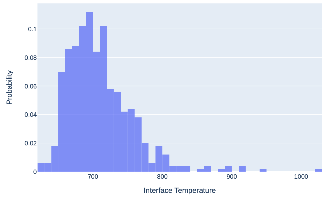
Figure 3: Histogram of $var element = document.getElementById("moose-equation-3097c8f3-802d-4ea0-8460-b0d3b92ec872");katex.render("T_i", element, {displayMode:false,throwOnError:false});$ when running with num_rows = 200 samples

We can also directly plot the random values sampled, i.e. the input distribution. These are shown in Figure 4.


python ../../contrib/moose/modules/stochastic_tools/python/make_histogram.py driver_out.json* -v sample_0 --xlabel 'Input Distribution' --output samples.pdf

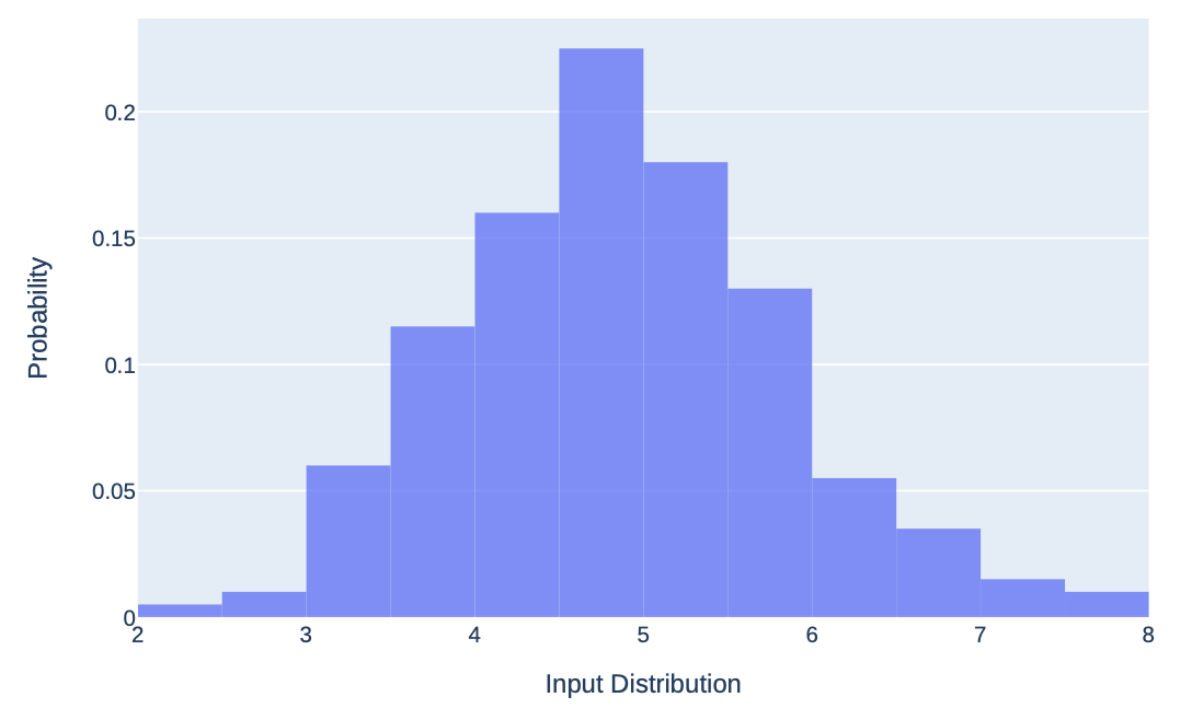
Figure 4: Actual sampled input distribution for $var element = document.getElementById("moose-equation-11344573-2426-46d1-93e4-4794da835686");katex.render("k_n", element, {displayMode:false,throwOnError:false});$

Because we added the the StatisticsReporter, we also have access to the mean, standard deviation, and confidence intervals automatically (of course, you could post-compute those as well). We can output this data as a table, using the visualize_statistics.py script.


python ../../contrib/moose/modules/stochastic_tools/python/visualize_statistics.py driver_out.json --markdown-table --names '{"storage_results:receive:nek_max_T":"Interface Temperature"}'

which will output


| Values                                 | MEAN                 | STDDEV              |
|:---------------------------------------|:---------------------|:--------------------|
| Interface Temperature (5.0%, 95.0%) CI | 714.4 (709.3, 719.8) | 45.1 (39.98, 50.22) |

We invite you to explore these plotting scripts and documentation in the STM, as this tutorial only scratches the surface with the simulations performed. You can make bar plots and many other data presentation formats.

Other Features

By default, when you run NekRS in a stochastic simulation, each individual run will write the NekRS solution to the same field files – <case>0.f*. These will all clobber eachother. If you want to preserve a unique output file for each of the NekRS runs, you can set write_fld_files = true in the [Problem] block, which will write output files labeled as a00case, a01case, ..., z98case, z99case, giving you 2574 possible output files.

Perturbing NekRS Parameters

In this example, we perturbed the thermal conductivity, but there are many other parameters which can be modified in NekRS via the udf.properties function. Table 1 summarizes the parameters which can be modified by the udf.properties function. Because NekRS simulations can be run with any number of passive scalars, the content and ordering will depend on how many scalars you have. So, to be as general as possible, we've written Table 1 assuming you have a simulation with 3 passive scalars.

Table 1: Commmon parameters to modify in NekRS via udf.properties

Parameter	How to Access
Coefficient on time derivative of 0th scalar equation	0th slot in `o_SProp`
Coefficient on time derivative of 1st scalar equation	1st slot in `o_SProp`
Coefficient on time derivative of 2nd scalar equation	2nd slot in `o_SProp`
Coefficient on diffusion operator of 0th scalar equation	3rd slot in `o_SProp`
Coefficient on diffusion operator of 1st scalar equation	4th slot in `o_SProp`
Coefficient on diffusion operator of 2nd scalar equation	5th slot in `o_SProp`
Fluid dynamic viscosity	0th slot in `o_UProp`
Fluid density	1st slot in `o_UProp`

Other quantities which you can perturb include:

Boundary conditions
Anything in a GPU kernel, such as momentum or heat source terms
Geometry

(tutorials/nek_stochastic/channel.i)

[Mesh]
  [box]
    type = GeneratedMeshGenerator
    dim = 3
    nx = 10
    ny = 4
    nz = 4
    xmin = 0.0
    xmax = 1.0
    ymin = 0.0
    ymax = 1.0
    zmin = 0.0
    zmax = 2.0
    bias_x = 1.2
    elem_type = HEX20
  []
  [rename]
    type = RenameBoundaryGenerator
    input = box
    old_boundary = '0 1 2 3 4 5'
    new_boundary = '1 2 3 4 5 6'
  []
[]

# The following blocks only exist here for testing purposes, to have some
# postprocessors we check with a CSVDiff test to ensure this tutorial
# stays up to date with future possible syntax changes in MOOSE.

[Problem]
  type = FEProblem
  solve = false
[]

[Executioner]
  type = Steady
[]

[Postprocessors]
  [area_left]
    type = AreaPostprocessor
    boundary = '5'
  []
  [area_right]
    type = AreaPostprocessor
    boundary = '3'
  []
[]

[Outputs]
  csv = true
  file_base = channel
[]

(tutorials/nek_stochastic/channel.par)

[OCCA]
  backend = CPU

[GENERAL]
  stopAt = numSteps
  numSteps = 400
  dt = 1.0
  timeStepper = tombo2
  writeControl = steps
  writeInterval = 500
  polynomialOrder = 5

[VELOCITY]
  solver = none

[PRESSURE]

[TEMPERATURE]
  rhoCp = 50.0
  boundaryTypeMap = insulated, insulated, t, insulated, flux, insulated
  residualTol = 1.0e-6

  # You should set the mean values for any material properties you are
  # perturbing, because these are used to initialize the elliptic solvers
  # for the entire simulation, and you want to use a reasonably representative
  # value here.
  conductivity = 5.0

(tutorials/nek_stochastic/channel.oudf)

void scalarDirichletConditions(bcData * bc)
{
  bc->s = 500.0;
}

void scalarNeumannConditions(bcData * bc)
{
  // note: when running with Cardinal, Cardinal will allocate the usrwrk
  // array. If running with NekRS standalone (e.g. nrsmpi), you need to
  // replace the usrwrk with some other value or allocate it youself from
  // the udf and populate it with values.
  bc->flux = bc->usrwrk[bc->idM];
}

(tutorials/nek_stochastic/channel.udf)

#include "udf.hpp"

void uservp(nrs_t *nrs, double time, occa::memory o_U, occa::memory o_S, occa::memory o_UProp, occa::memory o_SProp)
{
  if (!nrs->usrwrk)
    return;

  dfloat k = nrs->usrwrk[1 * nrs->fieldOffset + 0];

  // apply that value; in nekRS, the 0th slot in o_SProp represents the 'conductivity'
  // field in the par file
  auto mesh = nrs->cds->mesh[0];
  auto o_diff = o_SProp + 0 * nrs->fieldOffset * sizeof(dfloat);
  platform->linAlg->fill(mesh->Nlocal, k, o_diff);
}

void UDF_LoadKernels(occa::properties & kernelInfo)
{
}

void UDF_Setup(nrs_t *nrs)
{
  udf.properties = &uservp;

  auto mesh = nrs->cds->mesh[0];

  int n_gll_points = mesh->Np * mesh->Nelements;
  for (int n = 0; n < n_gll_points; ++n)
    nrs->cds->S[n + 0 * nrs->cds->fieldOffset[0]] = 500.0; // temperature
}

(tutorials/nek_stochastic/nek.i)

[Mesh]
  type = NekRSMesh
  boundary = '5'
[]

[Problem]
  type = NekRSProblem
  casename = 'channel'

  [FieldTransfers]
    [flux]
      type = NekBoundaryFlux
      direction = to_nek
      usrwrk_slot = 0
    []
    [temperature]
      type = NekFieldVariable
      field = temperature
      direction = from_nek
    []
  []

  [ScalarTransfers]
    [k]
      type = NekScalarValue
      direction = to_nek
      usrwrk_slot = 1
      output_postprocessor = k_from_stm
    []
  []
[]

[Executioner]
  type = Transient

  [TimeStepper]
    type = NekTimeStepper
  []
[]

[Postprocessors]
  [max_temp]
    type = NekVolumeExtremeValue
    field = temperature
  []
  [k_from_stm] # this will just print to the screen the value of k received
    type = Receiver
  []
  [expect_max_T]
    type = ParsedPostprocessor
    function = '1000.0 / k_from_stm + 500.0'
    pp_names = k_from_stm
  []
[]

[Outputs]
  csv = true
  hide = 'flux_integral'
[]

[Controls]
  [stm]
    type = SamplerReceiver
  []
[]

(tutorials/nek_stochastic/nek.i)

[Mesh]
  type = NekRSMesh
  boundary = '5'
[]

[Problem]
  type = NekRSProblem
  casename = 'channel'

  [FieldTransfers]
    [flux]
      type = NekBoundaryFlux
      direction = to_nek
      usrwrk_slot = 0
    []
    [temperature]
      type = NekFieldVariable
      field = temperature
      direction = from_nek
    []
  []

  [ScalarTransfers]
    [k]
      type = NekScalarValue
      direction = to_nek
      usrwrk_slot = 1
      output_postprocessor = k_from_stm
    []
  []
[]

[Executioner]
  type = Transient

  [TimeStepper]
    type = NekTimeStepper
  []
[]

[Postprocessors]
  [max_temp]
    type = NekVolumeExtremeValue
    field = temperature
  []
  [k_from_stm] # this will just print to the screen the value of k received
    type = Receiver
  []
  [expect_max_T]
    type = ParsedPostprocessor
    function = '1000.0 / k_from_stm + 500.0'
    pp_names = k_from_stm
  []
[]

[Outputs]
  csv = true
  hide = 'flux_integral'
[]

[Controls]
  [stm]
    type = SamplerReceiver
  []
[]

(tutorials/nek_stochastic/nek.i)

[Mesh]
  type = NekRSMesh
  boundary = '5'
[]

[Problem]
  type = NekRSProblem
  casename = 'channel'

  [FieldTransfers]
    [flux]
      type = NekBoundaryFlux
      direction = to_nek
      usrwrk_slot = 0
    []
    [temperature]
      type = NekFieldVariable
      field = temperature
      direction = from_nek
    []
  []

  [ScalarTransfers]
    [k]
      type = NekScalarValue
      direction = to_nek
      usrwrk_slot = 1
      output_postprocessor = k_from_stm
    []
  []
[]

[Executioner]
  type = Transient

  [TimeStepper]
    type = NekTimeStepper
  []
[]

[Postprocessors]
  [max_temp]
    type = NekVolumeExtremeValue
    field = temperature
  []
  [k_from_stm] # this will just print to the screen the value of k received
    type = Receiver
  []
  [expect_max_T]
    type = ParsedPostprocessor
    function = '1000.0 / k_from_stm + 500.0'
    pp_names = k_from_stm
  []
[]

[Outputs]
  csv = true
  hide = 'flux_integral'
[]

[Controls]
  [stm]
    type = SamplerReceiver
  []
[]

(tutorials/nek_stochastic/ht.i)

[Mesh]
  [box]
    type = GeneratedMeshGenerator
    dim = 3
    nx = 10
    ny = 10
    nz = 10
    xmin = -0.2
    xmax = 0.0
    ymin = 0.0
    ymax = 1.0
    zmin = 0.0
    zmax = 2.0
  []
[]

[Variables]
  [temperature]
    initial_condition = 500.0
  []
[]

[Kernels]
  [diffusion]
    type = HeatConduction
    variable = temperature
    diffusion_coefficient = thermal_conductivity
  []
[]

[BCs]
  [left]
    type = NeumannBC
    variable = temperature
    value = 1000.0
    boundary = 'left'
  []
  [interface]
    type = MatchedValueBC
    variable = temperature
    v = nek_temp
    boundary = 'right'
  []
[]

[AuxVariables]
  [flux]
    family = MONOMIAL
    order = CONSTANT
  []
  [nek_temp]
    initial_condition = 500.0
  []
[]

[AuxKernels]
  [flux]
    type = DiffusionFluxAux
    variable = flux
    diffusion_variable = temperature
    component = normal
    diffusivity = thermal_conductivity
    boundary = 'right'
  []
[]

[Materials]
  [k]
    type = GenericConstantMaterial
    prop_names = 'thermal_conductivity'
    prop_values = '1.5'
  []
[]

[Postprocessors]
  [flux_integral]
    type = SideIntegralVariablePostprocessor
    variable = flux
    boundary = 'right'
  []
[]

[Executioner]
  type = Transient
  dt = 10.0
  nl_abs_tol = 1e-8

  steady_state_detection = true
  steady_state_tolerance = 5e-4
  steady_state_start_time = 30.0
[]

[MultiApps]
  [nek]
    type = TransientMultiApp
    input_files = 'nek.i'
    sub_cycling = true
    execute_on = timestep_end
    wait_for_first_app_init = true
  []
[]

[Transfers]
  [temperature]
    type = MultiAppGeneralFieldNearestLocationTransfer
    source_variable = temperature
    from_multi_app = nek
    variable = nek_temp
  []
  [flux]
    type = MultiAppGeneralFieldNearestLocationTransfer
    source_variable = flux
    to_multi_app = nek
    variable = flux
    from_boundaries = 'right'
  []
  [flux_integral]
    type = MultiAppPostprocessorTransfer
    to_postprocessor = flux_integral
    from_postprocessor = flux_integral
    to_multi_app = nek
  []
  [get_qoi]
    type = MultiAppReporterTransfer
    from_multi_app = nek
    from_reporters = 'max_temp/value'
    to_reporters = 'receive/nek_max_T'
  []
[]

[Outputs]
  print_linear_residuals = false
  hide = 'flux_integral'
[]

[Reporters]
  [receive]
    type = ConstantReporter
    real_names = 'nek_max_T'

    # This value doesnt do anything - you just need to have a dummy here
    real_values = 0.0
  []
[]

(tutorials/nek_stochastic/ht.i)

[Mesh]
  [box]
    type = GeneratedMeshGenerator
    dim = 3
    nx = 10
    ny = 10
    nz = 10
    xmin = -0.2
    xmax = 0.0
    ymin = 0.0
    ymax = 1.0
    zmin = 0.0
    zmax = 2.0
  []
[]

[Variables]
  [temperature]
    initial_condition = 500.0
  []
[]

[Kernels]
  [diffusion]
    type = HeatConduction
    variable = temperature
    diffusion_coefficient = thermal_conductivity
  []
[]

[BCs]
  [left]
    type = NeumannBC
    variable = temperature
    value = 1000.0
    boundary = 'left'
  []
  [interface]
    type = MatchedValueBC
    variable = temperature
    v = nek_temp
    boundary = 'right'
  []
[]

[AuxVariables]
  [flux]
    family = MONOMIAL
    order = CONSTANT
  []
  [nek_temp]
    initial_condition = 500.0
  []
[]

[AuxKernels]
  [flux]
    type = DiffusionFluxAux
    variable = flux
    diffusion_variable = temperature
    component = normal
    diffusivity = thermal_conductivity
    boundary = 'right'
  []
[]

[Materials]
  [k]
    type = GenericConstantMaterial
    prop_names = 'thermal_conductivity'
    prop_values = '1.5'
  []
[]

[Postprocessors]
  [flux_integral]
    type = SideIntegralVariablePostprocessor
    variable = flux
    boundary = 'right'
  []
[]

[Executioner]
  type = Transient
  dt = 10.0
  nl_abs_tol = 1e-8

  steady_state_detection = true
  steady_state_tolerance = 5e-4
  steady_state_start_time = 30.0
[]

[MultiApps]
  [nek]
    type = TransientMultiApp
    input_files = 'nek.i'
    sub_cycling = true
    execute_on = timestep_end
    wait_for_first_app_init = true
  []
[]

[Transfers]
  [temperature]
    type = MultiAppGeneralFieldNearestLocationTransfer
    source_variable = temperature
    from_multi_app = nek
    variable = nek_temp
  []
  [flux]
    type = MultiAppGeneralFieldNearestLocationTransfer
    source_variable = flux
    to_multi_app = nek
    variable = flux
    from_boundaries = 'right'
  []
  [flux_integral]
    type = MultiAppPostprocessorTransfer
    to_postprocessor = flux_integral
    from_postprocessor = flux_integral
    to_multi_app = nek
  []
  [get_qoi]
    type = MultiAppReporterTransfer
    from_multi_app = nek
    from_reporters = 'max_temp/value'
    to_reporters = 'receive/nek_max_T'
  []
[]

[Outputs]
  print_linear_residuals = false
  hide = 'flux_integral'
[]

[Reporters]
  [receive]
    type = ConstantReporter
    real_names = 'nek_max_T'

    # This value doesnt do anything - you just need to have a dummy here
    real_values = 0.0
  []
[]

(tutorials/nek_stochastic/ht.i)

[Mesh]
  [box]
    type = GeneratedMeshGenerator
    dim = 3
    nx = 10
    ny = 10
    nz = 10
    xmin = -0.2
    xmax = 0.0
    ymin = 0.0
    ymax = 1.0
    zmin = 0.0
    zmax = 2.0
  []
[]

[Variables]
  [temperature]
    initial_condition = 500.0
  []
[]

[Kernels]
  [diffusion]
    type = HeatConduction
    variable = temperature
    diffusion_coefficient = thermal_conductivity
  []
[]

[BCs]
  [left]
    type = NeumannBC
    variable = temperature
    value = 1000.0
    boundary = 'left'
  []
  [interface]
    type = MatchedValueBC
    variable = temperature
    v = nek_temp
    boundary = 'right'
  []
[]

[AuxVariables]
  [flux]
    family = MONOMIAL
    order = CONSTANT
  []
  [nek_temp]
    initial_condition = 500.0
  []
[]

[AuxKernels]
  [flux]
    type = DiffusionFluxAux
    variable = flux
    diffusion_variable = temperature
    component = normal
    diffusivity = thermal_conductivity
    boundary = 'right'
  []
[]

[Materials]
  [k]
    type = GenericConstantMaterial
    prop_names = 'thermal_conductivity'
    prop_values = '1.5'
  []
[]

[Postprocessors]
  [flux_integral]
    type = SideIntegralVariablePostprocessor
    variable = flux
    boundary = 'right'
  []
[]

[Executioner]
  type = Transient
  dt = 10.0
  nl_abs_tol = 1e-8

  steady_state_detection = true
  steady_state_tolerance = 5e-4
  steady_state_start_time = 30.0
[]

[MultiApps]
  [nek]
    type = TransientMultiApp
    input_files = 'nek.i'
    sub_cycling = true
    execute_on = timestep_end
    wait_for_first_app_init = true
  []
[]

[Transfers]
  [temperature]
    type = MultiAppGeneralFieldNearestLocationTransfer
    source_variable = temperature
    from_multi_app = nek
    variable = nek_temp
  []
  [flux]
    type = MultiAppGeneralFieldNearestLocationTransfer
    source_variable = flux
    to_multi_app = nek
    variable = flux
    from_boundaries = 'right'
  []
  [flux_integral]
    type = MultiAppPostprocessorTransfer
    to_postprocessor = flux_integral
    from_postprocessor = flux_integral
    to_multi_app = nek
  []
  [get_qoi]
    type = MultiAppReporterTransfer
    from_multi_app = nek
    from_reporters = 'max_temp/value'
    to_reporters = 'receive/nek_max_T'
  []
[]

[Outputs]
  print_linear_residuals = false
  hide = 'flux_integral'
[]

[Reporters]
  [receive]
    type = ConstantReporter
    real_names = 'nek_max_T'

    # This value doesnt do anything - you just need to have a dummy here
    real_values = 0.0
  []
[]

(tutorials/nek_stochastic/driver.i)

[StochasticTools]
[]

[Distributions]
  [dist]
    type = Normal
    mean = 5.0
    standard_deviation = 1.0
  []
[]

[Samplers]
  [sample]
    type = MonteCarlo
    num_rows = 3
    distributions = 'dist'
  []
[]

[MultiApps]
  [ht]
    type = SamplerFullSolveMultiApp
    input_files = ht.i
    sampler = sample
    mode = batch-restore
    wait_for_first_app_init = true
  []
[]

[Transfers]
  [transer_random_inputs_to_nek]
    type = SamplerParameterTransfer
    to_multi_app = ht
    sampler = sample

    # you can send data down to arbitrarily-nested sub-apps
    parameters = 'nek:Problem/ScalarTransfers/k/value'
  []
  [results]
    type = SamplerReporterTransfer
    from_multi_app = ht
    sampler = sample
    stochastic_reporter = storage
    from_reporter = 'receive/nek_max_T'
  []
[]

[Reporters]
  [storage]
    type = StochasticMatrix
    sampler = sample
    parallel_type = ROOT
  []
  [stats]
    type = StatisticsReporter
    reporters = 'storage/results:receive:nek_max_T'
    compute = 'mean stddev'
    ci_method = 'percentile'
    ci_levels = '0.05 0.95'
  []
[]

[Outputs]
  execute_on = timestep_end
  [out]
    type = JSON
  []
[]

(tutorials/nek_stochastic/driver.i)

[StochasticTools]
[]

[Distributions]
  [dist]
    type = Normal
    mean = 5.0
    standard_deviation = 1.0
  []
[]

[Samplers]
  [sample]
    type = MonteCarlo
    num_rows = 3
    distributions = 'dist'
  []
[]

[MultiApps]
  [ht]
    type = SamplerFullSolveMultiApp
    input_files = ht.i
    sampler = sample
    mode = batch-restore
    wait_for_first_app_init = true
  []
[]

[Transfers]
  [transer_random_inputs_to_nek]
    type = SamplerParameterTransfer
    to_multi_app = ht
    sampler = sample

    # you can send data down to arbitrarily-nested sub-apps
    parameters = 'nek:Problem/ScalarTransfers/k/value'
  []
  [results]
    type = SamplerReporterTransfer
    from_multi_app = ht
    sampler = sample
    stochastic_reporter = storage
    from_reporter = 'receive/nek_max_T'
  []
[]

[Reporters]
  [storage]
    type = StochasticMatrix
    sampler = sample
    parallel_type = ROOT
  []
  [stats]
    type = StatisticsReporter
    reporters = 'storage/results:receive:nek_max_T'
    compute = 'mean stddev'
    ci_method = 'percentile'
    ci_levels = '0.05 0.95'
  []
[]

[Outputs]
  execute_on = timestep_end
  [out]
    type = JSON
  []
[]

Problem Setup
NekRS Model
Heat Conduction Model
Stochastic Tools Module
Summary
Execution and Postprocessing
Other Features
Perturbing NekRS Parameters