Converting CSG to CAD Geometry for Multiphysics
In this tutorial, you will learn how to:
Convert OpenMC CSG-based models to DAGMC using the Coreform Cubit CSG-to-CAD converter
Perform multiphysics feedback on a portion of the OpenMC model by coupling to finite element heat conduction
Run hybrid CSG + DAGMC OpenMC models with Cardinal
To access this tutorial,
cd cardinal/tutorials/csg_to_cad
This tutorial also requires you to download some mesh files from Box. Please download the files from the csg_to_cad folder here and place these files within tutorials/csg_to_cad.
To run this tutorial, you need to have built Cardinal with DAGMC support enabled, by setting export ENABLE_DAGMC=true.
Geometry and Computational Models
This model consists of a simplified version of the KRUSTY reactor. The neutronics model contains the fuel, heat pipes, and several layers of radial insulation and reflector materials. Simplified material compositions have been used, and many ex-core components have been removed for the sake of a simpler tutorial.
A conceptual image of the (i) fully-detailed KRUSTY model (background transparent image) and the simplified CSG models used in this tutorial (foreground) is shown below.
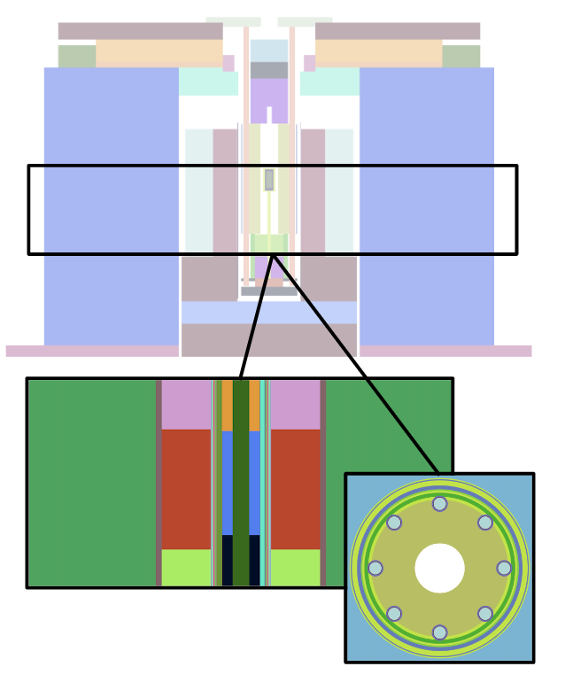
Figure 1: OpenMC CSG model with which we will start from
Converting CSG to CAD using Coreform Cubit
The OpenMC CAD adapter provides the capability to convert OpenMC cells to CAD parts in the form of a Cubit journal file that can be imported into Cubit. These CAD models can then be exported to various other CAD formats supported by Cubit (ACIS, IGES, STEP, etc.) or parts can be meshed for use in other simulations – as is the case in this tutorial.
OpenMC provides a plotting utility, which is useful for exploring CSG models, but it is limited to axis-aligned slices of the geometry. CAD and meshing utilities commonly support interactive rendering of parts, which is useful for debugging geometry problems as well as verifying the shape and/or placement of neutronics cells.
To generate a journal file of the KRUSTY model provided here with the CAD adapter, run the following command:
openmc_to_cad original_model.xml -w 1000 1000 1000 -c 1
This will produce two files, openmc.jou and openmc_cell1.jou, that contain the entire KRUSTY model and cell 1, the fuel region, respectively. It is interesting to view the full model in CAD, but we will only need the first cell for the purposes of this tutorial.
To open and import the full model in to Cubit, select the "Play journal file" button
Cubit> playback "openmc.jou"
The quotes around the file name in the block above are meaningful in Cubit's console and should not be omitted.
The model should then appear in Cubit.
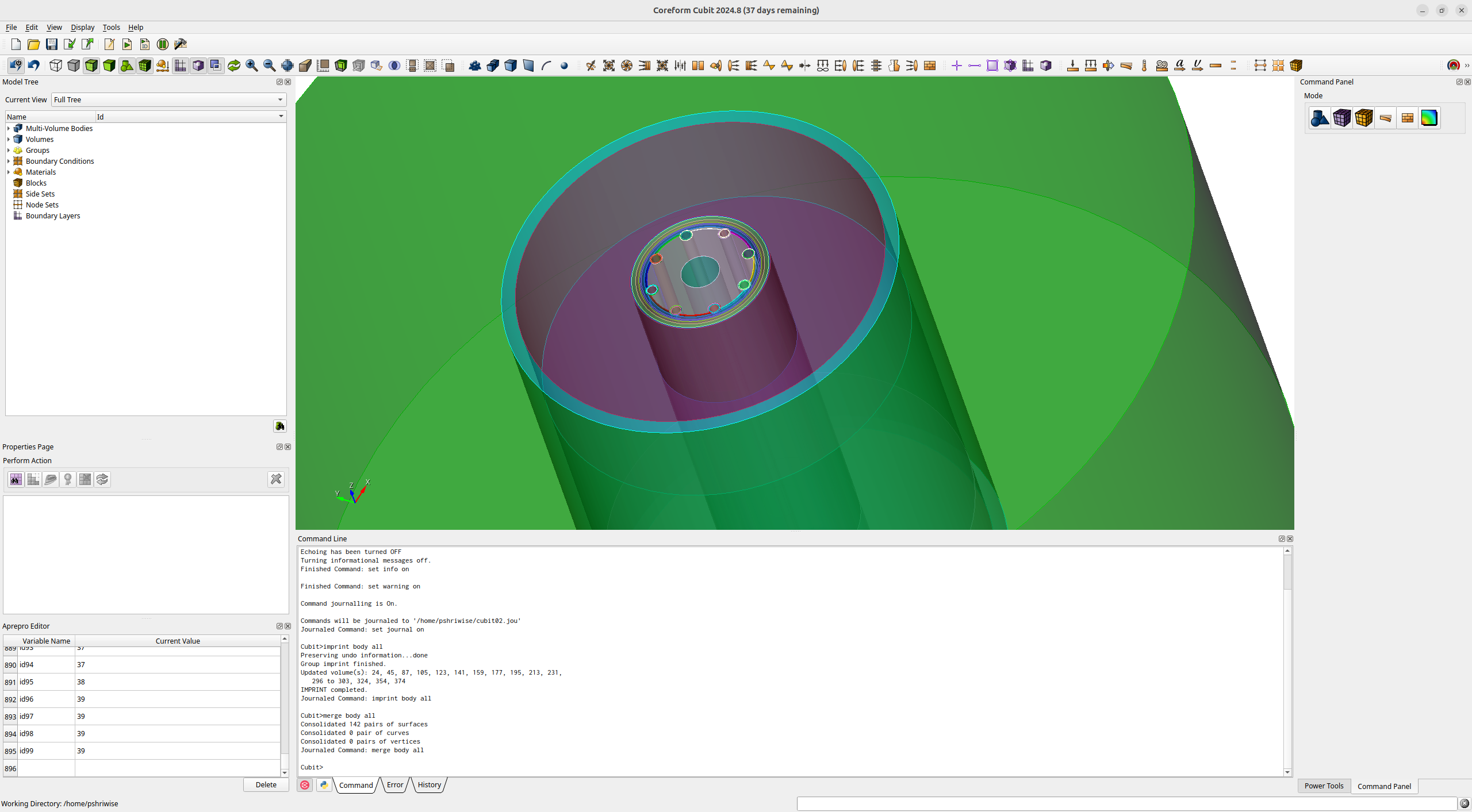
Figure 2: OpenMC CSG model, converted into CAD and loaded into Cubit
The model can then be examined for accuracy, with the material assignments appering as groups in the model tree.
The ability to interactively explore the model as CAD is extremely useful for visualization and debugging of a CSG model, which can be difficult to keep track of when relying on a mental model supported by 2D slices from native plotting utilities.
However, for this example we only need a single volume to couple heating in the center fuel volume (contained in the group labeled "mat:U-7.65Mo Fuel"). Let's instead import that single cell into Cubit.
Cubit> reset
Cubit> playback "openmc_cell1.jou"
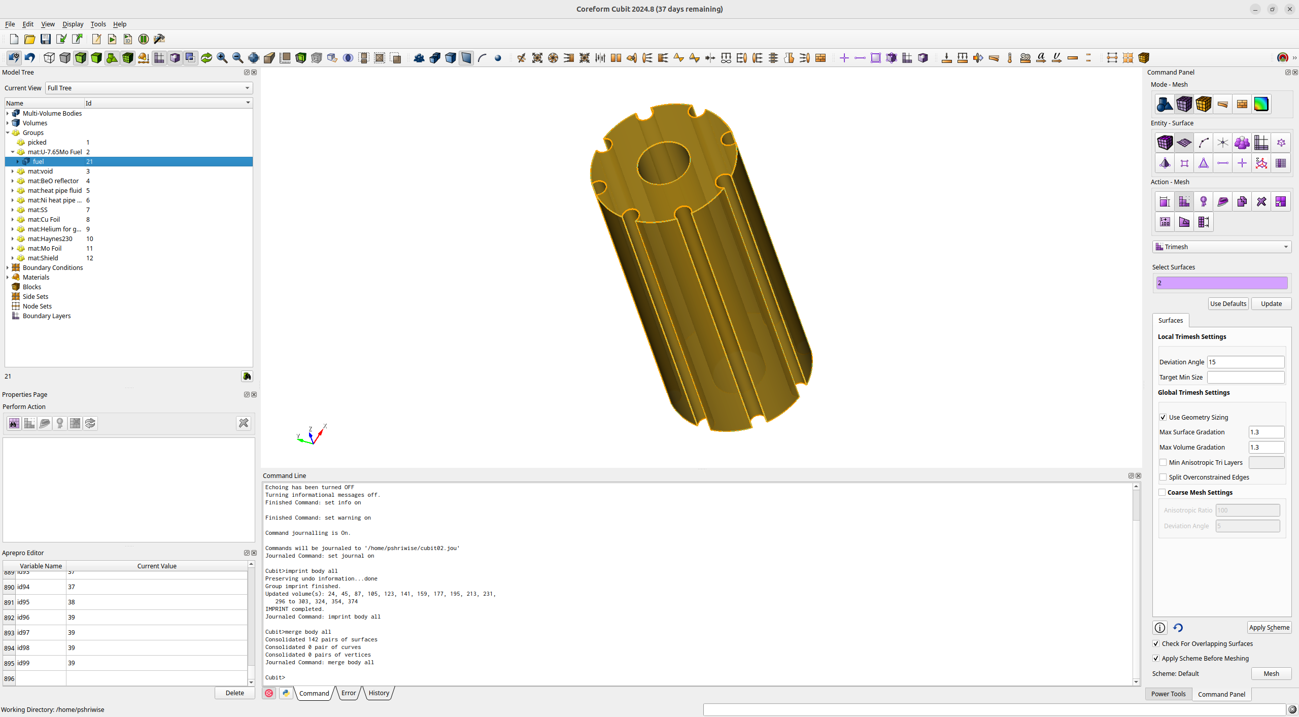
Figure 3: Fuel volume of the KRUSTY reactor imported into Cubit.
Next we'll create 2 meshes:
A surface mesh of triangle for the DAGMC geometry. This will represent the geometry boundaries for particle transport
A volumetric mesh for a heating tally and decomposition based on the temperature field produced by heat conduction in MOOSE.
Generate the DAGMC Surface Mesh
For the DAGMC mesh, we'll apply Cubit's trimesh scheme to all the surfaes of the fuel volume. This will produce a watertight mesh for particle transport. Normally the coarse mesh settings would be used to build the DAGMC mesh, but in this case we'll disable that setting to obtain triangles with a better aspect ratio for the tetrahedral mesh we'll create later.
Cubit> set trimesher coarse off
Cubit> set trimesher split overconstrained edges on
Cubit> surface all scheme trimesh
Cubit> mesh surface all
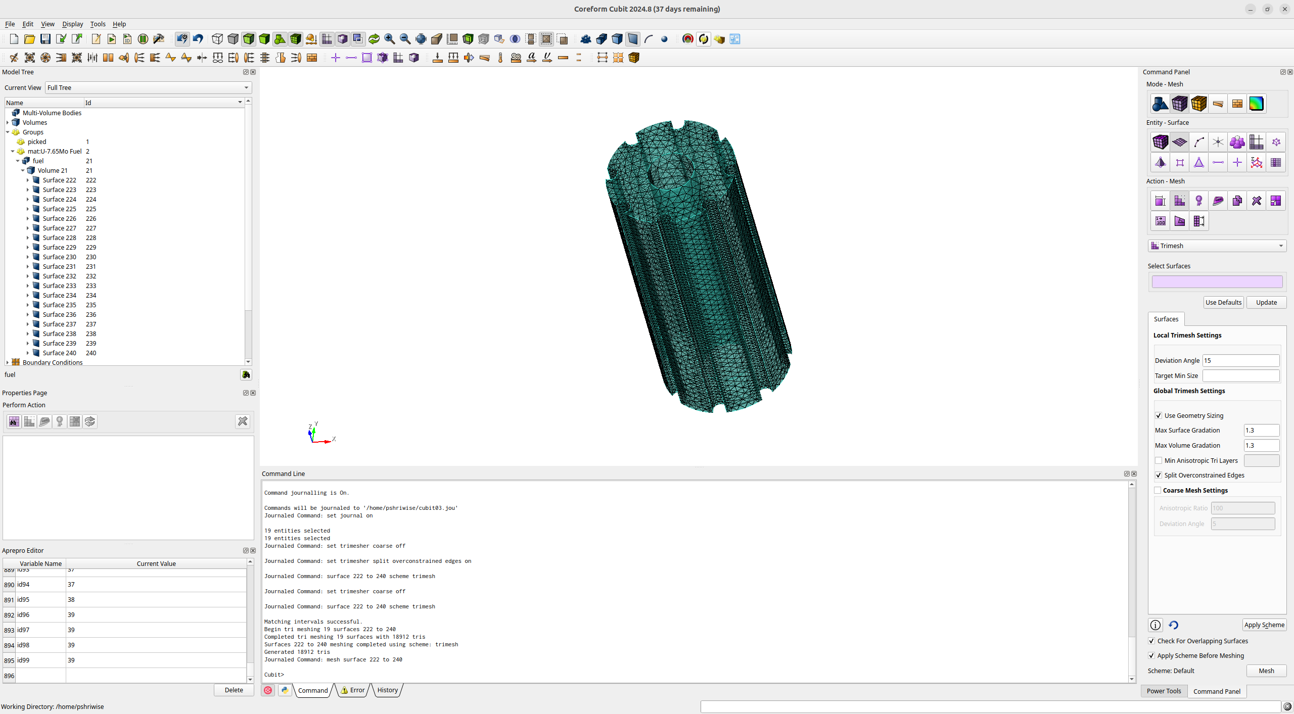
Figure 4: The surface mesh of the fuel volume.
Now that this is complete, we'll want to make sure the metadata converted from the OpenMC model is handled appropriately. To do this we'll use some capabilites from the DAGMC toolbar which can be added to Cubit. One of the capabilities is the conversion of group-based metadata to blocks and materials. We'll perform this conversion by clicking the button with the tooltip "Materials to Block Assignments".
Note: that this conversion can also be accomplished based on instructions found in previous Coreform Cubit webinars on modern DAGMC workflows.
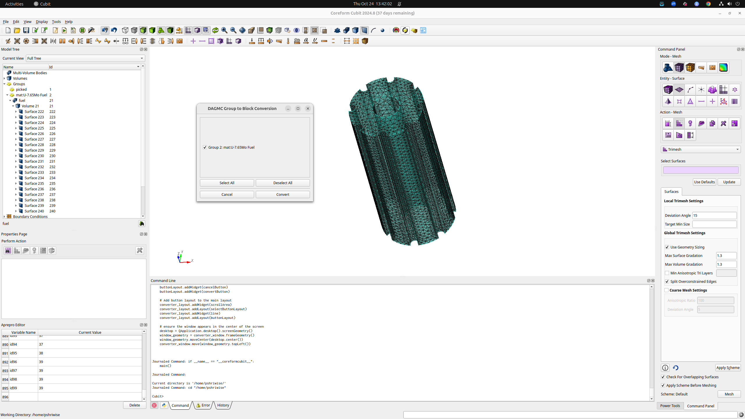
Figure 5: DAGMC group-based material assignments (legacy) to block assignments.
This mesh can now be exported to the .h5m format supported by DAGMC.
Cubit> export dagmc "krusty_fuel.h5m"
Note: This can also be accomplished in Cubit's export GUI.
Generate the Cardinal Mesh
When generating the Cardinal mesh, we want to ensure that the triangles of the DAGMC mesh correspond to the triangles used in the DAGMC mesh. Generating both meshes in Cubit allows us to guarantee that the boundaries of the two meshes are conformal. This mesh will be used to both tally heating in OpenMC and evaluate heat conductioon in MOOSE.
Cubit> set duplicate block elements on
Cubit> tetmesh tri all make block
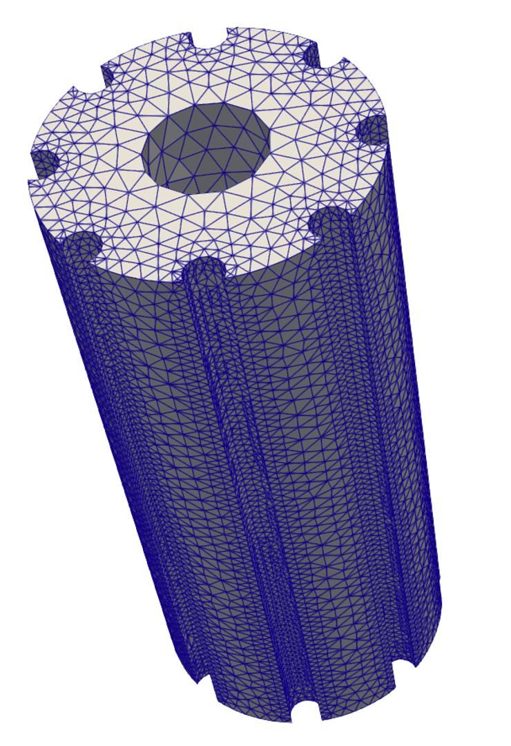
Figure 6: Tetrahedral mesh of the fuel volume.
Next, the mesh sideset "heat_pipes" can be added. Cardinal will expect to find on this sideset on the mesh.
Cubit> sideset 1 add surface 233 to 240
Cubit> sideset 1 name "heat_pipes"
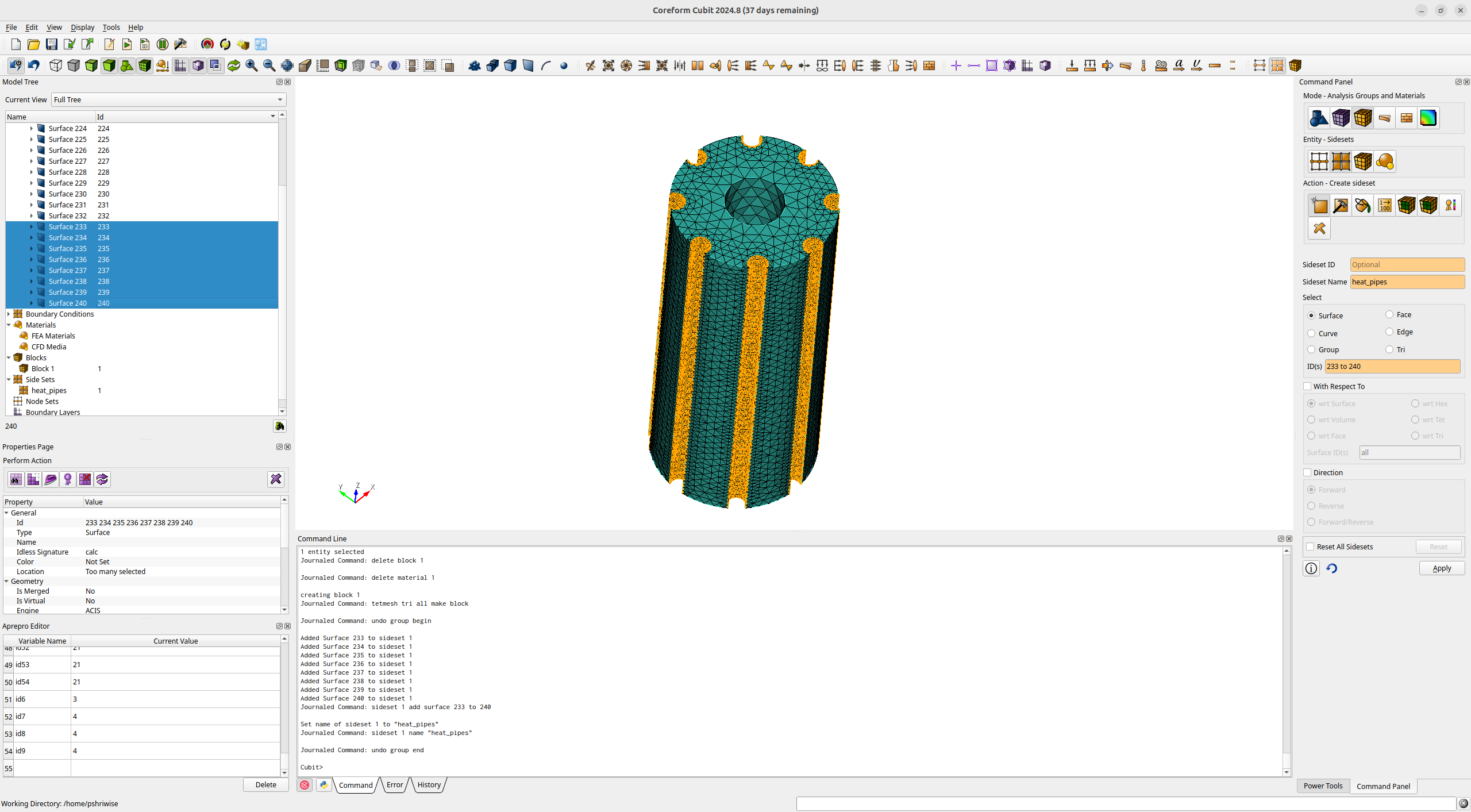
Figure 7: Generation of the sideset for Cardinal's heat conduction boundary condition.
This mesh can now be exported for use in multiphysics copuling.
Cubit> export mesh "/Users/pshriwise/krusty.e"
A different OpenMC model is needed to apply the DAGMC model generated, this is already present in the tutorial directory and will be used by Cardinal as it is set to the default filename expected by OpenMC ("model.xml"). This hybrid CSG/CAD model can also be produced by running the make_hybrid_model.py script.
Multiphysics Coupling
We have built a hybrid Computer Aided Design (CAD) and CSG model of the KRUSTY reactor in OpenMC, along with a volume mesh for tallying and solving heat conduction. In this section, we briefly describe the input files used to couple heat conduction to neutronics.
MOOSE Heat Conduction
We solve for the fuel temperature using the finite element method using MOOSE. We will solve using the volume mesh produced from Cubit. This mesh is identical to the mesh which OpenMC will use for tallying, but does not striclty need to be (it can be entirely different, and most other tutorials demonstrate this feature). But in this case, we will for simplicity use an identical mesh.
[Mesh<<<{"href": "../syntax/Mesh/index.html"}>>>]
  [fuel]
    type = FileMeshGenerator<<<{"description": "Read a mesh from a file.", "href": "../source/meshgenerators/FileMeshGenerator.html"}>>>
    file<<<{"description": "The filename to read."}>>> = krusty_fuel.e
  []
[]We will solve for temperature, with a variable T. The power density will be supplied by OpenMC, so we create a variable named power in this file in order to receive that field. The OpenMC tally will be a constant value in every mesh element, so we define this variable to match this basis.
[Variables<<<{"href": "../syntax/Variables/index.html"}>>>]
  [T]
  []
[]

[AuxVariables<<<{"href": "../syntax/AuxVariables/index.html"}>>>]
  [power]
    family<<<{"description": "Specifies the family of FE shape functions to use for this variable"}>>> = MONOMIAL
    order<<<{"description": "Specifies the order of the FE shape function to use for this variable (additional orders not listed are allowed)"}>>> = CONSTANT
  []
[]Next, we specify the governing equation and boundary conditions. We will solve for the steady-state temperature distribution
We use the HeatConduction and CoupledForce kernels to define the Laplacian kernel and the coupled power term, respectively. For boundary conditions, we apply a constant temperature of 800 on the surface of the heat pipes.
[Kernels<<<{"href": "../syntax/Kernels/index.html"}>>>]
  [heat_conduction]
    type = HeatConduction<<<{"description": "Diffusive heat conduction term $-\\nabla\\cdot(k\\nabla T)$ of the thermal energy conservation equation", "href": "../source/kernels/HeatConduction.html"}>>>
    variable<<<{"description": "The name of the variable that this residual object operates on"}>>> = T
  []
  [power]
    type = CoupledForce<<<{"description": "Implements a source term proportional to the value of a coupled variable. Weak form: $(\\psi_i, -\\sigma v)$.", "href": "../source/kernels/CoupledForce.html"}>>>
    variable<<<{"description": "The name of the variable that this residual object operates on"}>>> = T
    v<<<{"description": "The coupled variable which provides the force"}>>> = power
  []
[]

[BCs<<<{"href": "../syntax/BCs/index.html"}>>>]
  [surface]
    type = DirichletBC<<<{"description": "Imposes the essential boundary condition $u=g$, where $g$ is a constant, controllable value.", "href": "../source/bcs/DirichletBC.html"}>>>
    variable<<<{"description": "The name of the variable that this residual object operates on"}>>> = T
    boundary<<<{"description": "The list of boundary IDs from the mesh where this object applies"}>>> = 'heat_pipes'
    value<<<{"description": "Value of the BC"}>>> = 800
  []
[]

[Materials<<<{"href": "../syntax/Materials/index.html"}>>>]
  [k]
    type = GenericConstantMaterial<<<{"description": "Declares material properties based on names and values prescribed by input parameters.", "href": "../source/materials/GenericConstantMaterial.html"}>>>
    prop_names<<<{"description": "The names of the properties this material will have"}>>> = 'thermal_conductivity'
    prop_values<<<{"description": "The values associated with the named properties"}>>> = '0.1'
  []
[]Lastly, we need to specify a value for the thermal conductivity. We will set this to a constant value, for simplicity.
[Materials<<<{"href": "../syntax/Materials/index.html"}>>>]
  [k]
    type = GenericConstantMaterial<<<{"description": "Declares material properties based on names and values prescribed by input parameters.", "href": "../source/materials/GenericConstantMaterial.html"}>>>
    prop_names<<<{"description": "The names of the properties this material will have"}>>> = 'thermal_conductivity'
    prop_values<<<{"description": "The values associated with the named properties"}>>> = '0.1'
  []
[]Finally, we need to specify how to solve this equation. We will use a transient executioner, which will allow us to solve the equation multiple times. We also indicate the output file format (exodus). For the sake of normalizing the power we receive from OpenMC, we also add a postprocessor to compute the total integral of power - while we don't strictly need this because our meshes are identical between OpenMC and MOOSE for this problem, having this block here would be necessary if OpenMC and MOOSE were using different meshes, to guarantee power conservation.
[Postprocessors<<<{"href": "../syntax/Postprocessors/index.html"}>>>]
  [tally_integral]
    type = ElementIntegralVariablePostprocessor<<<{"description": "Computes a volume integral of the specified variable", "href": "../source/postprocessors/ElementIntegralVariablePostprocessor.html"}>>>
    variable<<<{"description": "The name of the variable that this object operates on"}>>> = power
    execute_on<<<{"description": "The list of flag(s) indicating when this object should be executed. For a description of each flag, see https://mooseframework.inl.gov/source/interfaces/SetupInterface.html."}>>> = transfer
  []
[]

[Executioner<<<{"href": "../syntax/Executioner/index.html"}>>>]
  type = Transient
[]

[Outputs<<<{"href": "../syntax/Outputs/index.html"}>>>]
  exodus<<<{"description": "Output the results using the default settings for Exodus output."}>>> = true
[]OpenMC Neutron Transport
Our input file to run OpenMC within a MOOSE simulation will look similar to the previous input file syntax. First, we now have a problem block to inform MOOSE to replace it's typical finite element solver with calls to OpenMC -eigenvalue runs. We will have temperature feedback to OpenMC on block 1, and we add two mesh tallies. This will tally the kappa_fission local power deposition and the flux from OpenMC and map them to the mesh used in the mesh block. Other settings in the problem block refer to how to normalize the tallies from OpenMC into meaningful engineering units (W/volume for heating terms, and neutrons/area/time for flux).
power = 3000

[Problem<<<{"href": "../syntax/Problem/index.html"}>>>]
  type = OpenMCCellAverageProblem
  power = ${power}

  temperature_blocks = '1'
  cell_level = 1

  skinner = skinner

  source_rate_normalization = 'kappa_fission'

  [Tallies<<<{"href": "../syntax/Problem/Tallies/index.html"}>>>]
    [mesh]
      type = MeshTally<<<{"description": "A class which implements unstructured mesh tallies.", "href": "../source/tallies/MeshTally.html"}>>>
      score<<<{"description": "Score(s) to use in the OpenMC tallies. If not specified, defaults to 'kappa_fission'"}>>> = 'kappa_fission flux'

      normalize_by_global_tally<<<{"description": "Whether to normalize local tallies by a global tally (true) or else by the sum of the local tally (false)"}>>> = false
    []
  []
[]

[Mesh<<<{"href": "../syntax/Mesh/index.html"}>>>]
  [fuel]
    type = FileMeshGenerator<<<{"description": "Read a mesh from a file.", "href": "../source/meshgenerators/FileMeshGenerator.html"}>>>
    file<<<{"description": "The filename to read."}>>> = krusty_fuel.e
  []
[]We will dynamically modify the OpenMC geometry by "skinning" with the MoabSkinner object. For simplicity, we will lump elements into new cells by contouring into 4 intervals between temperatures of 800 K and 1000 K.
[UserObjects<<<{"href": "../syntax/UserObjects/index.html"}>>>]
  [skinner]
    type = MoabSkinner<<<{"description": "Re-generate the OpenMC geometry on-the-fly according to changes in the mesh geometry and/or contours in temperature and density", "href": "../source/userobjects/MoabSkinner.html"}>>>
    temperature<<<{"description": "Temperature variable by which to bin elements"}>>> = temp
    n_temperature_bins<<<{"description": "Number of temperature bins"}>>> = 4
    temperature_min<<<{"description": "Lower bound of temperature bins"}>>> = 800
    temperature_max<<<{"description": "Upper bound of temperature bins"}>>> = 1000
    build_graveyard<<<{"description": "Whether to build a graveyard around the geometry"}>>> = true
  []
[]Next, we specify how to pass data between OpenMC and the finite element heat conduction solver in the fuel.i input file. We will run the heat conduction solver as a sub-application. On every time step, we will pass temperature (into OpenMC) and the heating tally (out of OpenMC) as listed in the transfers block. The other details listed in this section are details on the source/receiver variable names in each file and which postprocessors to use to ensure power conservation.
[MultiApps<<<{"href": "../syntax/MultiApps/index.html"}>>>]
  [conduction]
    type = TransientMultiApp<<<{"description": "MultiApp for performing coupled simulations with the parent and sub-application both progressing in time.", "href": "../source/multiapps/TransientMultiApp.html"}>>>
    input_files<<<{"description": "The input file for each App.  If this parameter only contains one input file it will be used for all of the Apps.  When using 'positions_from_file' it is also admissable to provide one input_file per file."}>>> = 'fuel.i'
    execute_on<<<{"description": "The list of flag(s) indicating when this object should be executed. For a description of each flag, see https://mooseframework.inl.gov/source/interfaces/SetupInterface.html."}>>> = timestep_end
  []
[]

[Transfers<<<{"href": "../syntax/Transfers/index.html"}>>>]
  [heat_source_from_openmc]
    type = MultiAppGeneralFieldShapeEvaluationTransfer<<<{"description": "Transfers field data at the MultiApp position using the finite element shape functions from the origin application.", "href": "../source/transfers/MultiAppGeneralFieldShapeEvaluationTransfer.html"}>>>
    to_multi_app<<<{"description": "The name of the MultiApp to transfer the data to"}>>> = conduction
    source_variable<<<{"description": "The variable to transfer from."}>>> = kappa_fission
    variable<<<{"description": "The auxiliary variable to store the transferred values in."}>>> = power
    from_postprocessors_to_be_preserved<<<{"description": "The name of the Postprocessor in the from-app to evaluate an adjusting factor."}>>> = tally_integral
    to_postprocessors_to_be_preserved<<<{"description": "The name of the Postprocessor in the to-app to evaluate an adjusting factor."}>>> = tally_integral
  []
  [temp_to_openmc]
    type = MultiAppGeneralFieldShapeEvaluationTransfer<<<{"description": "Transfers field data at the MultiApp position using the finite element shape functions from the origin application.", "href": "../source/transfers/MultiAppGeneralFieldShapeEvaluationTransfer.html"}>>>
    from_multi_app<<<{"description": "The name of the MultiApp to receive data from"}>>> = conduction
    variable<<<{"description": "The auxiliary variable to store the transferred values in."}>>> = temp
    source_variable<<<{"description": "The variable to transfer from."}>>> = T
  []
[]Next, we set some initial conditions, since OpenMC will run first. We set a constant initial temperature of 800 K. Lastly, we indicate the run settings - we will run OpenMC three times, and output all results to Exodus.
[ICs<<<{"href": "../syntax/Cardinal/ICs/index.html"}>>>]
  [temp]
    type = ConstantIC<<<{"description": "Sets a constant field value.", "href": "../source/ics/ConstantIC.html"}>>>
    variable<<<{"description": "The variable this initial condition is supposed to provide values for."}>>> = temp
    value<<<{"description": "The value to be set in IC"}>>> = 800
  []
  [power]
    type = ConstantIC<<<{"description": "Sets a constant field value.", "href": "../source/ics/ConstantIC.html"}>>>
    variable<<<{"description": "The variable this initial condition is supposed to provide values for."}>>> = kappa_fission
    value<<<{"description": "The value to be set in IC"}>>> = ${fparse power/1.865e+03}
  []
[]

[Postprocessors<<<{"href": "../syntax/Postprocessors/index.html"}>>>]
  [tally_integral]
    type = ElementIntegralVariablePostprocessor<<<{"description": "Computes a volume integral of the specified variable", "href": "../source/postprocessors/ElementIntegralVariablePostprocessor.html"}>>>
    variable<<<{"description": "The name of the variable that this object operates on"}>>> = kappa_fission
    execute_on<<<{"description": "The list of flag(s) indicating when this object should be executed. For a description of each flag, see https://mooseframework.inl.gov/source/interfaces/SetupInterface.html."}>>> = 'initial transfer timestep_end'
  []
[]

[Executioner<<<{"href": "../syntax/Executioner/index.html"}>>>]
  type = Transient
  num_steps = 3
[]

[Outputs<<<{"href": "../syntax/Outputs/index.html"}>>>]
  exodus<<<{"description": "Output the results using the default settings for Exodus output."}>>> = true
[]Execution and Postprocessing
To run the coupled calculation,
mpiexec -np 2 cardinal-opt -i openmc.i --n-threads=2
This will run both MOOSE and OpenMC with 2 MPI processes and 2 OpenMP threads per rank. To run the simulation faster, you can increase the parallel processes/threads, or simply decrease the number of particles used in OpenMC. When the simulation has completed, you will have created a number of different output files:
openmc_out.e: Exodus output file with all variables in theopenmc.ifileopenmc_out_conduction0.e: Exodus output file with all variables in thefuel.ifile
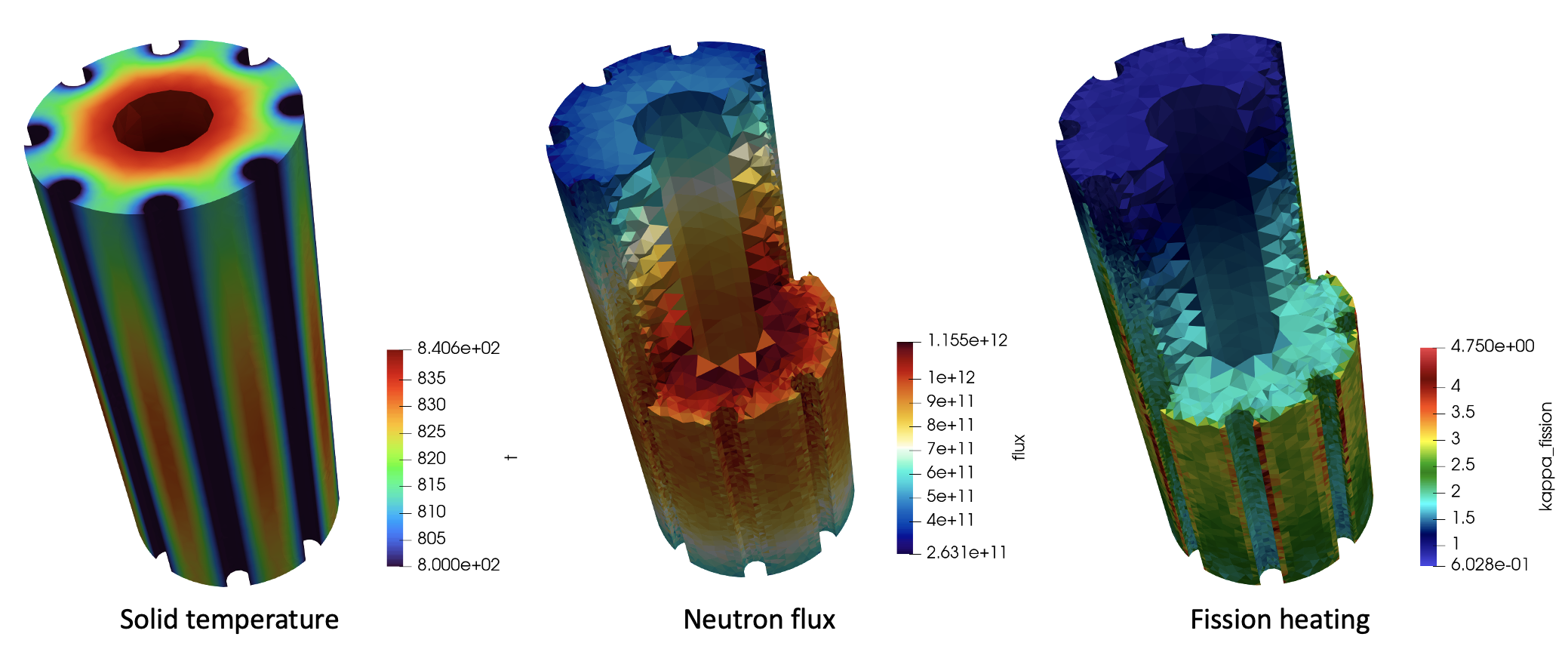
Figure 8: Solid temperature (left), and OpenMC predictions for neutron flux (middle) and fission heating (right). This simulation is run with an increased number of particles compared to the tutorial files in order to obtain well-converged results.