Assessing Convergence
In this tutorial, you will learn how to:
Use helper scripts in Cardinal to assess convergence of the OpenMC solution and of a general MOOSE application
To access this tutorial, enter the following directory and then also generate the necessary mesh file,
cd cardinal/tutorials/gas_compact
cardinal-opt -i mesh.i --mesh-only
This tutorial provides a description of several helper scripts available in the cardinal/scripts directory that can be used for:
Determining an appropriate number of inactive batches for OpenMC to ensure convergence of the fission source and eigenvalue
Determining an appropriate cell discretization in OpenMC in the presence of thermal feedback
Determining appropriate mesh convergence of a generic MOOSE application
Convergence of the OpenMC Model
When building an OpenMC model, there are several parameters that affect the convergence:
Number of inactive batches, which must be sufficiently high to ensure that the fission distribution and are converged before beginning to tally in the active batches
Number of active batches, which must be sufficiently high to reach a desired uncertainty in and the tallies
Cell discretization, such as the number of axial layers in a pincell-type geometry or the number of radial cell divisions in a pebble-type geometry, such that the actual temperature and density distributions passed into OpenMC are converged in terms of the effect on the Monte Carlo transport physics
To ensure that a sufficient number of active batches are used, we recommend using the trigger system in the OpenMC wrapping, which will terminate the number of active batches once reaching a desired uncertainty in and/or the kappa-fission tally. To determine an appropriate nuber of inactive batches and a cell discretization, Cardinal contains several helper scripts. This tutorial describes how to use these scripts.
You will need to install OpenMC's Python API to use the OpenMC convergence helper scripts. Please follow the instructions here.
Inactive Batches
To determine an appropriate number of inactive batches, you can use the scripts/inactive_study.py script. To run this script, you need:
A Python script that creates your OpenMC model for you; this Python script must take
-sas a boolean argument that indicates a Shannon entropy mesh will be added, and-n <layers>to indicate the number of cell divisions to createA Cardinal input file that runs your OpenMC model given some imposed temperature and density distribution
For example, to run an inactive cycle study for the model developed for the gas compact tutorial, we would run:
cd tutorials/gas_compact
python ../../scripts/inactive_study.py -i unit_cell -input openmc.i
since the Python script used to generate the OpenMC model is named unit_cell.py and our Cardinal input file is named openmc.i. You should edit the beginning of the inactive_study.py script to select the number of cell layers and number of inactive cycles to consider:
# This script runs the OpenMC wrapping for a number of axial layer discretizations
# in order to determine how many inactive cycles are needed to converge both the
# Shannon entropy and k. This script is run with:
#
# python inactive_study.py -i <script_name> -input <file_name> --method=<method> [--window_length=<LENGTH>]  [-n-threads <n_threads>]
#
# - The script used to create the OpenMC model is named <script_name>.py.
#   This script MUST accept '-s' as an argument to add a Shannon entropy mesh
#   AND '-n' to set the number of layers.
#   Please consult the tutorials for examples if you're unsure of how to do this.
# - The Cardinal input file to run is named <file_name>.
# - By default, the number of threads is taken as the maximum on your system.
#   Otherwise, you can set it by providing -n-threads <n_threads>.
# - A method to assist the user in detecting convergence is <method>, which
#   can be specified from all, half, window, or none (default).
#   If the window method is selected, then window_length
#   must also be specified.
#
# This script will create plots named <script_name>_k_<layers>.pdf and
# <script_name>_entropy_<layers>.pdf in a sub-directory named inactive_study/.

# Whether to use saved statepoint files to just generate plots, skipping transport solves
use_saved_statepoints = False

# Number of cell layers to consider
n_layers = [5, 10]

# Number of inactive batches to run
n_inactive = 100

# Number of inactive batches to average over to draw average-k line
averaging_batches = 100

# ------------------------------------------------------------------------------ #

from argparse import ArgumentParser
import multiprocessing
import matplotlib
import matplotlib.pyplot as plt
import numpy as np
import openmc
import sys
import os

matplotlib.rcParams.update({'font.size': 14})
colors = ['firebrick', 'orangered', 'darkorange', 'goldenrod', 'forestgreen', \
          'lightseagreen', 'steelblue', 'slateblue']

program_description = ("Script for determining required number of inactive batches "
                       "for an OpenMC model divided into a number of layers")
ap = ArgumentParser(description=program_description)

ap.add_argument('-i', dest='script_name', type=str, required=True,
                help='Name of the OpenMC python script to run (without .py extension)')
ap.add_argument('-n-threads', dest='n_threads', type=int,
                default=multiprocessing.cpu_count(), help='Number of threads to run Cardinal with')
ap.add_argument('-input', dest='input_file', type=str, required=True,
                help='Name of the Cardinal input file to run')
ap.add_argument('--method', dest = 'method', choices =['all','half','window','none'], default='none',
                help = 'The method to estimate the number of sufficient inactive batches to discard before tallying in k-eigenvalue mode. ' +
                'This number is determined by the first batch at which a running average of the Shannon Entropy falls within the standard ' +
                'deviation of the run. Options are all, half, and window; all uses all batches, half uses the last half of the batches, and ' +
                'window uses a user-specified number. Additionally, none can be specified if the feature is undesired.')
ap.add_argument('--window_length', dest = 'window_length', type = int,
                help =' When the window method is selected, the window length must be specified. The window length is a number of batches '
                ' before the current batch to use when computing the running average and standard deviation.')
args = ap.parse_args()

# variable to be used in logic for which way to detect steady state
method = args.method

if (args.method == 'window' and args.window_length == None):
    raise TypeError('The method specified was window, but window_length = None. Please specify --window_length = LENGTH, where LENGTH is an integer')
else:
    if (args.method == 'window'):
        window_length = args.window_length

input_file = args.input_file
script_name = args.script_name + ".py"
file_path = os.path.realpath(__file__)
file_dir, file_name = os.path.split(file_path)
exec_dir, file_name = os.path.split(file_dir)

# Number of active batches to run (a small number, inconsequential for this case)
n_active = 10

# methods to look for, in order of preference
methods = ['opt', 'devel', 'oprof', 'dbg']
exec_name = ''
for i in methods:
  if (os.path.exists(exec_dir + "/cardinal-" + i)):
    exec_name = exec_dir + "/cardinal-" + i
    break

if (exec_name == ''):
  raise ValueError("No Cardinal executable was found!")

# create directory to write plots if not already existing
if (not os.path.exists(os.getcwd() + '/inactive_study')):
  os.makedirs(os.getcwd() + '/inactive_study')

entropy = []
k = []
k_generation_avg = []
n_batches = n_inactive + n_active

max_entropy = sys.float_info.min
min_entropy = sys.float_info.max
max_k = sys.float_info.min
min_k = sys.float_info.max

for n in n_layers:
    new_sp_filename = 'inactive_study/statepoint_' + str(n) + '_layers.h5'

    if ((not use_saved_statepoints) or (not os.path.exists(new_sp_filename))):
        # Generate a new set of OpenMC XML files
        os.system("python " + script_name + " -s -n " + str(n))

        # Run Cardinal
        os.system(exec_name + " -i " + input_file + \
            " Problem/inactive_batches=" + str(n_inactive) + \
            " Problem/batches=" + str(n_batches) + \
            " Problem/max_batches=" + str(n_batches) + \
            " MultiApps/active='' Transfers/active='' Executioner/num_steps=1" + \
            " --n-threads=" + str(args.n_threads))

        # Copy the statepoint to a separate file for later plotting
        os.system('cp statepoint.' + str(n_batches) + '.h5 ' + new_sp_filename)

    with openmc.StatePoint(new_sp_filename) as sp:
        entropy.append(sp.entropy)
        k.append(sp.k_generation)
        max_entropy = max(np.max(sp.entropy[:n_inactive][:]), max_entropy)
        min_entropy = min(np.min(sp.entropy[:n_inactive][:]), min_entropy)
        max_k = max(np.max(sp.k_generation[:n_inactive][:]), max_k)
        min_k = min(np.min(sp.k_generation[:n_inactive][:]), min_k)

        averaging_k = sp.k_generation[(n_inactive - averaging_batches):n_inactive]
        k_generation_avg.append(sum(averaging_k) / len(averaging_k))

entropy_range = max_entropy - min_entropy
for i in range(len(n_layers)):
    nl = n_layers[i]
    fig, ax = plt.subplots()
    ax.plot(entropy[i][:n_inactive][:], label='{0:.0f} layers'.format(nl), color=colors[i])
    ax.set_xlabel('Inactive Batch')
    ax.set_ylabel('Shannon Entropy')
    ax.set_ylim([min_entropy - 0.05 * entropy_range, max_entropy + 0.05 * entropy_range])
    plt.grid()
    plt.legend(loc='upper right')
    plt.savefig('inactive_study/' + args.script_name + '_entropy' + str(nl) + '.pdf', bbox_inches='tight')
    plt.close()

for i in range(len(n_layers)):
    nl = n_layers[i]
    fig, ax = plt.subplots()
    ax.plot(k[i][:n_inactive][:], label='{0:.0f} layers'.format(nl), color=colors[i])
    plt.axhline(y=k_generation_avg[i], color='k', linestyle='-')

    ax.set_xlabel('Inactive Batch')
    ax.set_ylabel('$k$')
    ax.set_ylim([min_k, max_k])
    plt.grid()
    plt.legend(loc='lower right')
    plt.savefig('inactive_study/' + args.script_name + '_k' + str(nl) + '.pdf', bbox_inches='tight')
    plt.close()

if (method != 'none'):
    # loop over each layer (index i) and report inactive batch (index j) that satisfies
    # convergence criteria for the selected method
    for i in range(len(n_layers)):
        nl = n_layers[i]
        print("\nLayers: ", nl)
        print("----------------------")
        start = 1
        if (method == "window"):
          start = window_length

        for j in range(start, len(entropy[i])):
            if (method == "window"):
                # moving window, of constant width
                window = entropy[i][(j - window_length):j]
            elif (method == "half"):
                # Brown (2006) "On the Use of Shannon Entropy of the Fission Distribution for
                # Assessing Convergence of Monte Carlo Criticality Calculations"
                # window is half of the previous cycles
                idx = int(np.floor(j/2))
                window = entropy[i][idx:j]
            else:
                # window is all previous cycles
                window = entropy[i][0:j]

            window_mean = np.average(window)
            window_dev = np.std(window)
            window_low = window_mean - window_dev
            window_high = window_mean + window_dev
            extra_str = "    "
            if (entropy[i][j] <= window_high and entropy[i][j] >= window_low):
                extra_str = "--> "

            print(extra_str + "Inactive batch: {:6d} Entropy: {:.6f} Window mean: {:.6f} +/- {:.6f}".format(j, entropy[i][j], window_mean, window_dev))
    print("--> indicates batch which satisfies method. DOES NOT necessarily indicate a converged fission source.")
When the script finishes running, plots of Shannon entropy and , along with the saved statepoint files from the simulations, will be available in a directory named inactive_study. Below are shown example images of the Shannon entropy and plots. If a method to detect convergence of the fission source is supplied (the default is none), then the script will report whether the chosen metric succeeded or not. Note, there could be various factors affecting whether the metric succeeded or not, and based on user choices, it is possible for a metric to succeed when more batches or more particles per batch are truly needed. These metrics should be considered along side inspection of the plots of the Shannon Entropy, which typically takes longer than the eigenvalue to converge. Having a converged fission source is important so that when the active batches begin tallying, there is no contamination from the source's initial guess impacting the tallies.
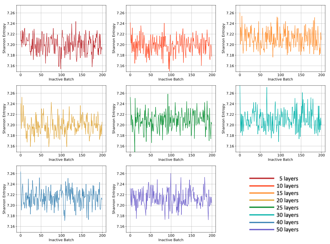
Figure 1: Example plots that are generated as part of the inactive study, showing Shannon entropy as a function of inactive batch and number of cell divisions
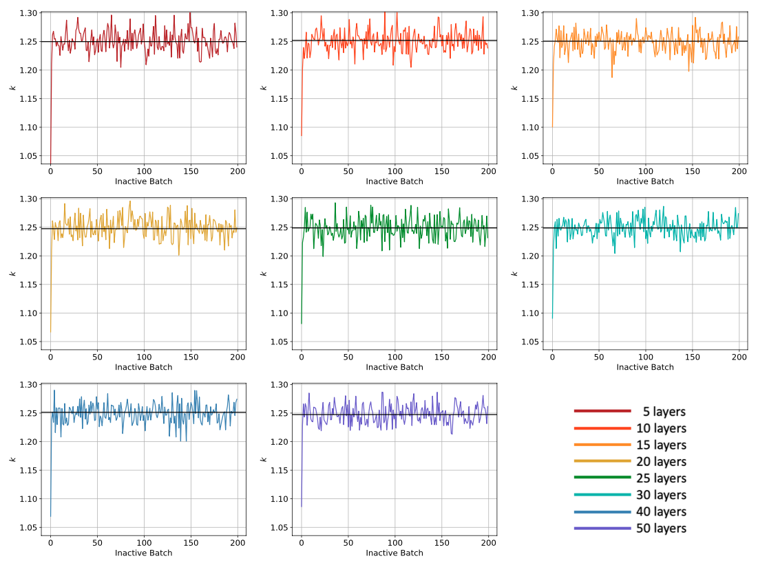
Figure 2: Example plots that are generated as part of the inactive study, showing as a function of inactive batch and number of cell divisions; the horizontal line shows the average of over the last 100 cycles
Cell Discretization
To determine an appropriate cell discretization, you can use the scripts/layers_study.py script. To run this script, you need:
A Python script that creates your OpenMC for you; this Python script must take
-n <layers>to indicate the number of cell divisions to createA Cardinal input file that runs your OpenMC model given some imposed temperature and density distribution
In addition, your Cardinal input file must contain a number of postprocessors, user objects, and vector postprocessors to process the solution to extract the various scalar and averaged quantities used in the convergence study. In the [Problem] block, you must set outputs = 'unrelaxed_tally_std_dev'. You will also need to copy and paste the following into your input file:
[Postprocessors]
  [max_tally_rel_err]
    type = TallyRelativeError
    value_type = max
  []
  [k]
    type = KEigenvalue
  []
  [k_std_dev]
    type = KEigenvalue
    output = 'std_dev'
  []
  [max_power]
    type = ElementExtremeValue
    variable = heat_source
    value_type = max
    block = 2
  []
  [min_power]
    type = ElementExtremeValue
    variable = heat_source
    value_type = min
    block = 2
  []

  [proxy_max_power_std_dev]
    type = ElementExtremeValue
    variable = unrelaxed_tally_std_dev
    proxy_variable = heat_source
    value_type = max
    block = 2
  []
  [proxy_min_power_std_dev]
    type = ElementExtremeValue
    variable = unrelaxed_tally_std_dev
    proxy_variable = heat_source
    value_type = min
    block = 2
  []
[]

[UserObjects]
  [average_power_axial]
    type = LayeredAverage
    variable = heat_source
    direction = z
    block = 2
  []
[]

[VectorPostprocessors]
  [power_avg]
    type = SpatialUserObjectVectorPostprocessor
    userobject = average_power_axial
  []
[]
When copying the above into your input file, be sure to update the block for the various power postprocessors and user objects to be the blocks on which the heat source is defined, as well as the direction for the LayeredAverage.
For example, to run a cell discretization study for the model developed for the gas compact tutorial, we would run:
cd tutorials/gas_compact
python ../../scripts/layers_study.py -i unit_cell -input openmc.i
since the Python script used to generate the OpenMC model is named unit_cell.py and our Cardinal input file is named openmc.i. You should edit the beginning of the layers_study.py script to select the number of cell layers, number of inactive cycles, and maxium number of active cycles:
# This script runs the OpenMC wrapping for a number of cell layer discretizations
# in order to determine how many layers are needed to converge both the power
# distribution and k. Your OpenMC model should include triggers for k and/or
# the tallies in order to control when the OpenMC simulation should terminate.
# This script should be run with:
#
# python layers_study.py -i <script_name> -input <file_name> [-n-threads <n_threads>]
#
# - the script used to create the OpenMC model is named <script_name>.py;
#   this script MUST accept '-n' to set the number of layers; please consult
#   the tutorials for examples if you're unsure of how to do this
# - the Cardinal input file to run is named <file_name>
# - by default, the number of threads is taken as the maximum on your system;
#   otherwise, you can set it by providing -n-threads <n_threads>
#
# This script will create plots of the maximum power, minimum power, radially-
# averaged power, and k as a function of the number of layers in the
# layers_study/ directory.
#
# NOTE: Your input file must also contain a number of postprocessors and user
# objects to generate these plots. Please consult the documentation for this
# script to determine which objects you need in your input file:
# https://cardinal.cels.anl.gov/tutorials/convergence.html

import math

# Whether to use saved statepoint files to just generate plots, skipping transport solves
use_saved_statepoints = False

# Number of cell layers to consider
n_layers = [10, 20, 30, 40, 50]

# Number of inactive batches to run
n_inactive = 25

# Minimum number of active batches to run
n_active = 5

# Maximum number of active batches to run
n_max_active = 1000

# Interval with which to check the triggers
batch_interval = 2

# Height of the domain, to be used for plotting the averaged heat source
h = 1.6

# Average power density, for displaying percent changes in power in terms of
# the average (otherwise, large changes in low-power nodes can distort the sense
# of convergence)
average_power_density = 9.605e7

# ------------------------------------------------------------------------------ #

from argparse import ArgumentParser
import multiprocessing
import matplotlib
import matplotlib.pyplot as plt
import pandas
import numpy as np
import openmc
import csv
import sys
import os

matplotlib.rcParams.update({'font.size': 14})
colors = ['firebrick', 'orangered', 'darkorange', 'goldenrod', 'forestgreen', \
          'lightseagreen', 'steelblue', 'slateblue']

program_description = ("Script for determining required number of cell divisions "
                       "for an OpenMC model")
ap = ArgumentParser(description=program_description)

ap.add_argument('-i', dest='script_name', type=str,
                help='Name of the OpenMC python script to run (without .py extension)')
ap.add_argument('-n-threads', dest='n_threads', type=int,
                default=multiprocessing.cpu_count(), help='Number of threads to run Cardinal with')
ap.add_argument('-input', dest='input_file', type=str,
                help='Name of the Cardinal input file to run')

args = ap.parse_args()

input_file = args.input_file
script_name = args.script_name + ".py"
file_path = os.path.realpath(__file__)
file_dir, file_name = os.path.split(file_path)
exec_dir, file_name = os.path.split(file_dir)

# methods to look for, in order of preference
methods = ['opt', 'devel', 'oprof', 'dbg']
exec_name = ''
for i in methods:
  if (os.path.exists(exec_dir + "/cardinal-" + i)):
    exec_name = exec_dir + "/cardinal-" + i
    break

if (exec_name == ''):
  raise ValueError("No Cardinal executable was found!")

# create directory to write plots if not already existing
if (not os.path.exists(os.getcwd() + '/layers_study')):
  os.makedirs(os.getcwd() + '/layers_study')

nl = len(n_layers)

k = np.empty([nl])
k_std_dev = np.empty([nl])
max_power = np.empty([nl])
min_power = np.empty([nl])
max_power_std_dev = np.empty([nl])
min_power_std_dev = np.empty([nl])
q = np.empty([nl, max(n_layers)])

for i in range(nl):
    n = n_layers[i]
    file_base = "layers_study/openmc_" + str(n) + "_out"
    output_csv = file_base + ".csv"

    if ((not use_saved_statepoints) or (not os.path.exists(output_csv))):
        # Generate a new set of OpenMC XML files
        os.system("python " + script_name + " -n " + str(n))

        # Run Cardinal
        os.system(exec_name + " -i " + input_file + \
            " UserObjects/average_power_axial/num_layers=" + str(n) + \
            " Problem/inactive_batches=" + str(n_inactive) + \
            " Problem/batches=" + str(n_active + n_inactive) + \
            " Problem/max_batches=" + str(n_max_active + n_inactive) + \
            " Problem/batch_interval=" + str(batch_interval) + \
            " MultiApps/active='' Transfers/active='' Executioner/num_steps=1" + \
            " Outputs/file_base=" + file_base + \
            " --n-threads=" + str(args.n_threads))

    # Read the postprocessor values from the CSV output
    data = pandas.read_csv(output_csv)
    k[i] = data.at[1, 'k']
    k_std_dev[i] = data.at[1, 'k_std_dev']
    max_power[i] = data.at[1, 'max_power']
    min_power[i] = data.at[1, 'min_power']
    max_power_std_dev[i] = data.at[1, 'proxy_max_power_std_dev']
    min_power_std_dev[i] = data.at[1, 'proxy_min_power_std_dev']

# Print the percent change in max/min powers
for i in range(1, nl):
    n = n_layers[i]
    print('Layers: ' + str(n) + ':')
    print('\tPercent change in max power: ' + str(abs(max_power[i] - max_power[i - 1]) / max_power[i - 1] * 100))
    print('\tPercent change in min power: ' + str(abs(min_power[i] - min_power[i - 1]) / min_power[i - 1] * 100))
    print('\tPercent change in max power (rel. to avg.): ' + str(abs(max_power[i] - max_power[i - 1]) / average_power_density * 100))
    print('\tPercent change in min power (rel. to avg.): ' + str(abs(min_power[i] - min_power[i - 1]) / average_power_density * 100))

fig, ax = plt.subplots()
plt.errorbar(n_layers, max_power, yerr=max_power_std_dev, fmt='.r', capsize=3.0, marker='o', linestyle='-', color='r')
ax.set_xlabel('Axial Layers')
ax.set_ylabel('Maximum Power (W/m$^3$)')
plt.grid()
plt.savefig('layers_study/' + args.script_name + '_max_power_layers.pdf', bbox_inches='tight')
plt.close()

fig, ax = plt.subplots()
plt.errorbar(n_layers, min_power, yerr=min_power_std_dev, fmt='.b', capsize=3.0, marker='o', linestyle='-', color='b')
ax.set_xlabel('Axial Layers')
ax.set_ylabel('Minimum Power (W/m$^3$)')
plt.grid()
plt.savefig('layers_study/' + args.script_name + '_min_power_layers.pdf', bbox_inches='tight')
plt.close()

fig, ax = plt.subplots()
plt.errorbar(n_layers, k, yerr=k_std_dev, fmt='.k', capsize=3.0, marker='o', color='k', linestyle = '-')
plt.xlabel('Axial Layers')
plt.ylabel('$k$')
plt.grid()
plt.savefig('layers_study/' + args.script_name + '_k_layers.pdf', bbox_inches='tight')
plt.close()

fig, ax = plt.subplots()
for l in range(nl):
    i = n_layers[l]
    power_file = "layers_study/openmc_" + str(i) + "_out_power_avg_0001.csv"

    q = []
    with open(power_file) as f:
        reader = csv.reader(f)
        next(reader) # skip header
        for row in reader:
            q.append(float(row[0]))

    dz = h / i
    z = np.linspace(dz / 2.0, h - dz / 2.0, i)
    plt.plot(z, q, label='{} layers'.format(i), color=colors[l], marker='o', markersize=2.0)

plt.xlabel('Distance from Inlet (m)')
plt.ylabel('Power (W/m$^3$)')
plt.grid()
plt.legend(loc='lower center', ncol=2)
plt.savefig('layers_study/' + args.script_name + '_layers_q.pdf', bbox_inches='tight')
plt.close()
When the script finishes running, plots of the maximum power, minimum power, , and the axial power distribution, along with the saved CSV output from the simulations, will be available in a directory named layers_study. Below are shown example images of these quantities as a function of the cell discretization. You would then select the cell discretization scheme to be the point at which the changes in power and are sufficiently converged.
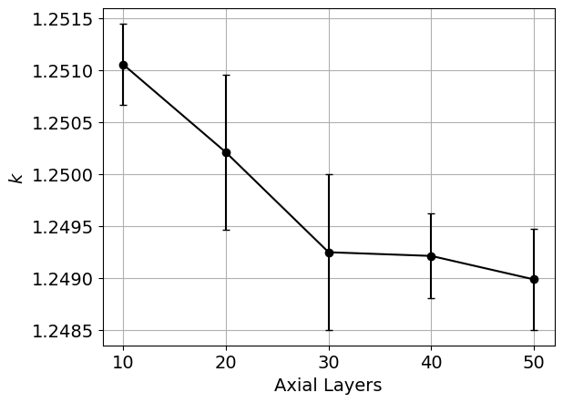
Figure 3: Example plot that is generated as part of the cell discretization study, showing as a function of the cell discretization
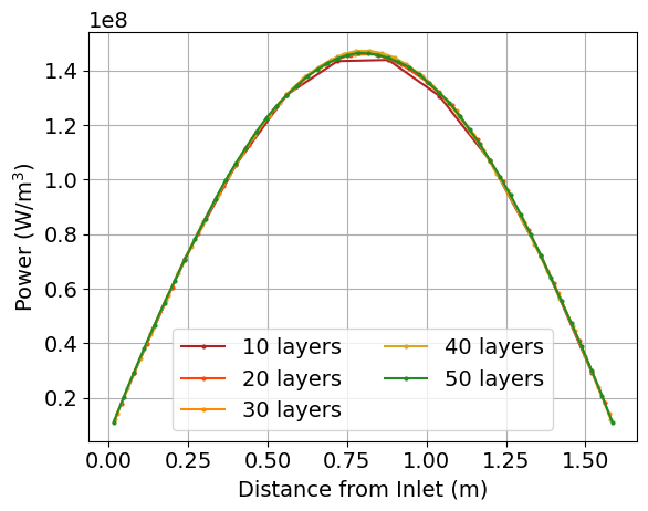
Figure 4: Example plot that is generated as part of the cell discretization study, showing the radially-averaged power distribution as a function of the cell discretization
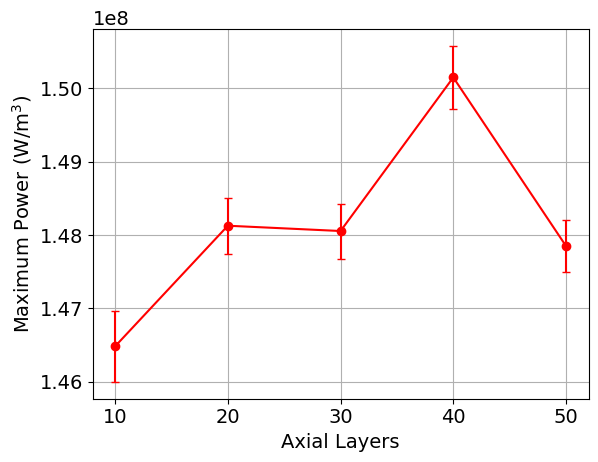
Figure 5: Example plot that is generated as part of the cell discretization study, showing the maximum power as a function of the cell discretization
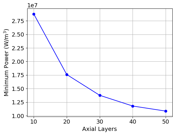
Figure 6: Example plot that is generated as part of the cell discretization study, showing the minimum power as a function of the cell discretization