Step 1: Flow Through a Channel
Complete input file for this step: 01_flow_channel.i
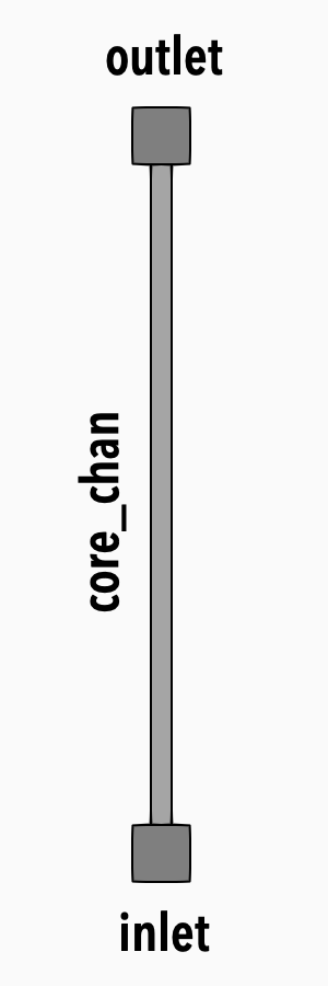
Figure 1: Model diagram
In the first step of this tutorial, we will setup a flow channel with mass flow rate inlet boundary condition and pressure outlet boundary condition.
We start by specifying several model parameters at the beginning of the input file
Simulation Parameters
We define inlet temperature T_in, inlet mass flow rate m_dot_in and pressure press parameters. These values will be used in the input file. It is a good practice to setup input files this way, because if a change is needed one can do it in a single location rather then hunting for all the right occurrences. This will become very important when input files get large.
T_in = 300. # K
m_dot_in = 1e-2 # kg/s
press = 10e5 # Pa
It is a good habit to include the units we are assuming in case our input file will be used by other people.
Note: THM is using SI units: kg, m, s, K.
Fluid Properties
In our model, we will be circulating helium in tubes, so we need to add a top-level [FluidProperties] block into the input file. In this block, we define all fluids that will be used by the flow components.
To model the helium gas, we will use the ideal gas equation of state. To do so, we will put the following block inside the [FluidProperties] block.
[FluidProperties<<<{"href": "../../../../syntax/FluidProperties/index.html"}>>>]
  [he]
    type = IdealGasFluidProperties<<<{"description": "Fluid properties for an ideal gas", "href": "../../../../source/fluidproperties/IdealGasFluidProperties.html"}>>>
    molar_mass<<<{"description": "Constant molar mass of the fluid (kg/mol)"}>>> = 4e-3
    gamma<<<{"description": "gamma value (cp/cv)"}>>> = 1.67
    k<<<{"description": "Thermal conductivity, W/(m-K)"}>>> = 0.2556
    mu<<<{"description": "Dynamic viscosity, Pa.s"}>>> = 3.22639e-5
  []
[]
Closures
Closure relations are provided through objects created in a [Closures] block. We define a set of closures of type Closures1PhaseTHM with default options, which will be used by our flow channel component:
[Closures<<<{"href": "../../../../syntax/Closures/index.html"}>>>]
  [thm_closures]
    type = Closures1PhaseTHM<<<{"description": "Closures for 1-phase flow channels", "href": "../../../../source/closures/Closures1PhaseTHM.html"}>>>
  []
[]
Flow Channel
The heart of all input files is the top-level [Components] block. Components represent pieces of a model, including physical pieces such as pipes, turbo-machinery, etc., and intangible pieces that add physics, like boundary conditions or source terms. They are like LEGO bricks which when put together they build up the overall simulation.
The first component we introduce is the FlowChannel1Phase component which represents a channel with single-phase flow.
[Components<<<{"href": "../../../../syntax/Components/index.html"}>>>]
  [core_chan]
    type = FlowChannel1Phase<<<{"description": "1-phase 1D flow channel", "href": "../../../../source/components/FlowChannel1Phase.html"}>>>
    position<<<{"description": "Start position of axis in 3-D space [m]"}>>> = '0 0 0'
    orientation<<<{"description": "Direction of flow channel from start position to end position (no need to normalize). For curved flow channels, it is the (tangent) direction at the start position."}>>> = '0 0 1'
    length<<<{"description": "Length of each axial section [m]"}>>> = 1
    n_elems<<<{"description": "Number of elements in each axial section"}>>> = 25
    A<<<{"description": "Area of the flow channel, can be a constant or a function"}>>> = 7.2548e-3
    D_h<<<{"description": "Hydraulic diameter [m]"}>>> = 7.0636e-2
  []
[]
The position parameter is a location in 3D space where the flow channel starts. The orientation parameter is the directional vector (in 3 dimensions) of the channel relative to the position parameter. The length parameter is the length of the channel. The n_elems parameter describes the number of elements that will be created for the mesh that supports the channel. The A and D_h parameters are the cross-sectional area and the hydraulic diameter of the flow channel. Note that the Darcy friction factor f_D is calculated by the closure set.
Every flow channel defines a subdomain block with its name and two boundaries. They are named flow_channel_name:in and flow_channel_name:out and refer to the start and the end of the flow channel, respectively. This will be useful later for connecting components together and setting up other objects like postprocessors.
Note: The flow_channel_name:in and flow_channel_name:out are only referring to the geometry of the channel. The actual flow direction will be determined by the physics and the boundary conditions connected to each end, i.e. flow_channel_name:in can be a flow outlet.
Boundary Conditions
Every flow channel has to be connected to either a boundary condition or a junction. If it is not, the code will detect it and report an error.
In this part of the tutorial we will look at connecting boundary conditions – junctions will be covered later. To connect a boundary condition to a flow channel we use the input parameter. The value we assign into it will be the name of the side of the flow channel (see the above note).
Inlet
For the channel inlet, we prescribe a mass flow rate and temperature boundary condition. The component expects two required parameters: m_dot and T. We use the simulation parameters we defined earlier at the beginning of this step, so the block will look like this:
[Components<<<{"href": "../../../../syntax/Components/index.html"}>>>]
  [inlet]
    type = InletMassFlowRateTemperature1Phase<<<{"description": "Boundary condition with prescribed mass flow rate and temperature for 1-phase flow channels.", "href": "../../../../source/components/InletMassFlowRateTemperature1Phase.html"}>>>
    input<<<{"description": "Name of the input"}>>> = 'core_chan:in'
    m_dot<<<{"description": "Prescribed mass flow rate [kg/s]"}>>> = ${m_dot_in}
    T<<<{"description": "Prescribed temperature [K]"}>>> = ${T_in}
  []
[]
Outlet
For the channel outlet, we prescribe pressure boundary condition and we use our press parameter to specify the pressure via a p parameter.
[Components<<<{"href": "../../../../syntax/Components/index.html"}>>>]
  [outlet]
    type = Outlet1Phase<<<{"description": "Boundary condition with prescribed pressure for 1-phase flow channels.", "href": "../../../../source/components/Outlet1Phase.html"}>>>
    input<<<{"description": "Name of the input"}>>> = 'core_chan:out'
    p<<<{"description": "Prescribed pressure [Pa]"}>>> = ${press}
  []
[]
Global Parameters
In [GlobalParams] block, we prescribe parameters that are global to the whole simulation.
The following parameter should be almost always included in your input file. It enables the full slope reconstruction in the underlying rDG scheme.
rdg_slope_reconstruction = full
If initial conditions are the same for the whole simulation, it is convenient to place them in this block. This is the case in this tutorial, so we will do so by including the following parameters in the [GlobalParams] block:
initial_p = ${press}
initial_vel = 0.0001
initial_T = ${T_in}
The closures parameter is used to specify the name of a closures object, so we pass the name we gave to the closures object we created in the Closures block:
closures = thm_closures
Since we will be using helium gas in almost all flow components, we can place the following in the [GlobalParams] block as well:
fp = he
This will make sure that all flow components will pick the helium gas, unless they will be directed otherwise.
Tip: Place the [GlobalParams] at the top of the input file for visibility.
Postprocessors
The postprocessor system comes from the MOOSE framework. Postprocessors are single Real values computed at different locations like blocks, sides, etc., or at different mesh entities like nodes or elements. There can also be postprocessors that are not associated with any mesh entities (like a postprocessor to output time step size, etc.).
In our model, we will add the following postprocessors to compute the pressure drop across the flow channel:
core_p_infor monitoring core inlet pressure[Postprocessors<<<{"href": "../../../../syntax/Postprocessors/index.html"}>>>] [core_p_in] type = SideAverageValue<<<{"description": "Computes the average value of a variable on a sideset. Note that this cannot be used on the centerline of an axisymmetric model.", "href": "../../../../source/postprocessors/SideAverageValue.html"}>>> boundary<<<{"description": "The list of boundary IDs from the mesh where this object applies"}>>> = core_chan:in variable<<<{"description": "The name of the variable which this postprocessor integrates"}>>> = p [] []core_p_outfor monitoring core outlet pressure[Postprocessors<<<{"href": "../../../../syntax/Postprocessors/index.html"}>>>] [core_p_out] type = SideAverageValue<<<{"description": "Computes the average value of a variable on a sideset. Note that this cannot be used on the centerline of an axisymmetric model.", "href": "../../../../source/postprocessors/SideAverageValue.html"}>>> boundary<<<{"description": "The list of boundary IDs from the mesh where this object applies"}>>> = core_chan:out variable<<<{"description": "The name of the variable which this postprocessor integrates"}>>> = p [] []core_delta_pfor monitoring the core pressure drop[Postprocessors<<<{"href": "../../../../syntax/Postprocessors/index.html"}>>>] [core_delta_p] type = ParsedPostprocessor<<<{"description": "Computes a parsed expression with post-processors", "href": "../../../../source/postprocessors/ParsedPostprocessor.html"}>>> pp_names<<<{"description": "Post-processors arguments"}>>> = 'core_p_in core_p_out' expression<<<{"description": "function expression"}>>> = 'core_p_in - core_p_out' [] []
The first two postprocessors are of SideAverageValue type which means they are computed on a side. The side is specified via the boundary parameter, and both postprocessors operate on the pressure variable p. Then we use a ParsedPostProcessor to compute the difference.
Executioner
This top-level block describes how the simulation will be executed.
[Executioner<<<{"href": "../../../../syntax/Executioner/index.html"}>>>]
  type = Transient
  solve_type = NEWTON
  line_search = basic

  start_time = 0
  end_time = 1000
  dt = 10

  petsc_options_iname = '-pc_type'
  petsc_options_value = 'lu'

  nl_rel_tol = 1e-8
  nl_abs_tol = 1e-8
  nl_max_its = 25
[]
The Transient type says that we will be solving multiple time steps starting from start_time and running until end_time with time step size (dt) of 10.
The line_search = basic and solve_type = NEWTON should be always present in this block when running a THM-based code. It is also advised to use the following PETSc options: petsc_options_iname = '-pc_type' and petsc_options_value = 'lu'. Their exact explanation is beyond the scope of this tutorial.
The nl_rel_tol, nl_abs_tol, and nl_max_its are parameters to decide if the non-linear solver converged and their meaning is relative and absolute tolerance and maximum number of non-linear iterations, respectively.
Outputs
By default, MOOSE will only produce an output to terminal.
For visualizing the obtained solution, we need to enable an output to a file or files. The most useful output is stored in an ExodusII file format and can be enabled by:
[Outputs<<<{"href": "../../../../syntax/Outputs/index.html"}>>>]
  exodus<<<{"description": "Output the results using the default settings for Exodus output."}>>> = true

  [console]
    type = Console<<<{"description": "Object for screen output.", "href": "../../../../source/outputs/Console.html"}>>>
    max_rows<<<{"description": "The maximum number of postprocessor/scalar values displayed on screen during a timestep (set to 0 for unlimited)"}>>> = 1
    outlier_variable_norms<<<{"description": "If true, outlier variable norms will be printed after each solve"}>>> = false
  []
  print_linear_residuals<<<{"description": "Enable printing of linear residuals to the screen (Console)"}>>> = false
[]
Notes
This is a typical input file structure of a THM-based code. All input files will be more or less similar to this.