Brayton Cycle
Introduction
The Brayton cycle is the ideal thermodynamic cycle for gas-turbine engines. Usually, it is used in an open system, where gas is drawn in from the environment and exhausted back into the environment. However, for some analyses, it is simpler to analyze the system as if it were a closed system that cycles the same working fluid in a closed loop, which can be done without significant loss of accuracy. Here we discuss how both open and closed cycles can be modeled.
In its simplest form, a Brayton cycle requires the following elements:
A heat source to add thermal energy to the working gas,
A heat sink to remove thermal energy from the working gas (in an open system, exhaust into the environment serves this function),
A compressor to compress the working gas, and
A turbine to expand the working gas.
Usually, the compressor and turbine are operated on the same shaft. In steady operation, the work the turbine provides to the shaft is partially consumed by the compressor when it applies work to the working fluid. The remainder can be used for the application's purposes, like electricity generation via a generator on the shaft. In practice, when starting up a Brayton engine, the turbine is not yet applying work to the shaft, and thus the compressor is not functioning either. Thus, a motor is used to drive the shaft until the cycle can sustain itself.
Example
Now an example will be given, first discussing the commonalities between the open and closed cycles and then describing the differences in the following sections.
The turbo-machinery setup for this example consists of a shaft, motor, compressor, turbine, and generator. The Shaft component connects them and specifies the initial shaft speed (here equal to zero since we are starting from rest):
[Components<<<{"href": "../../../../syntax/Components/index.html"}>>>]
  [shaft]
    type = Shaft<<<{"description": "Component that connects torque of turbomachinery components", "href": "../../../../source/components/Shaft.html"}>>>
    connected_components<<<{"description": "Names of the connected components"}>>> = 'motor compressor turbine generator'
    initial_speed<<<{"description": "Initial shaft speed"}>>> = ${speed_initial}
  []
[]
As mentioned previously, when starting up, a motor is needed, so we use ShaftConnectedMotor:
[Components<<<{"href": "../../../../syntax/Components/index.html"}>>>]
  [motor]
    type = ShaftConnectedMotor<<<{"description": "Motor to drive a shaft component", "href": "../../../../source/components/ShaftConnectedMotor.html"}>>>
    inertia<<<{"description": "Moment of inertia from the motor [N-m]"}>>> = ${I_motor}
    torque<<<{"description": "Driving torque supplied by the motor [kg-m^2]"}>>> = motor_torque_fn
  []
[]
The function chosen here is a linear ramp up from zero and back down to zero,
This is accomplished with a PiecewiseLinear function:
[Functions<<<{"href": "../../../../syntax/Functions/index.html"}>>>]
  [motor_torque_time_fn]
    type = PiecewiseLinear<<<{"description": "Linearly interpolates between pairs of x-y data", "href": "../../../../source/functions/PiecewiseLinear.html"}>>>
    x<<<{"description": "The abscissa values"}>>> = '0 ${t1} ${t2}'
    y<<<{"description": "The ordinate values"}>>> = '0 ${motor_torque_max} 0'
  []
[]
However, we cannot use this function directly because ShaftConnectedMotor treats the time coordinate in its functions as the shaft speed. Therefore we use control logic as follows, which controls a constant-value function to drop the time coordinate:
[Functions<<<{"href": "../../../../syntax/Functions/index.html"}>>>]
  [motor_torque_fn]
    type = ConstantFunction<<<{"description": "A function that returns a constant value as defined by an input parameter.", "href": "../../../../source/functions/ConstantFunction.html"}>>>
    value<<<{"description": "The constant value"}>>> = 0 # controlled
  []
[]
[ControlLogic<<<{"href": "../../../../syntax/ControlLogic/index.html"}>>>]
[get_motor_torque_control]
type = GetFunctionValueControl<<<{"description": "Sets a ControlData named 'value' with the value of a function", "href": "../../../../source/controllogic/GetFunctionValueControl.html"}>>>
function<<<{"description": "The name of the function prescribing a value."}>>> = motor_torque_time_fn
[]
[set_motor_torque_control]
type = SetRealValueControl<<<{"description": "Control object that reads a Real value computed by the control logic system and sets it into a specified MOOSE object parameter(s)", "href": "../../../../source/controllogic/SetRealValueControl.html"}>>>
parameter<<<{"description": "The input parameter(s) to control"}>>> = Functions/motor_torque_fn/value
value<<<{"description": "The name of control data to be set into the input parameter."}>>> = get_motor_torque_control:value
[]
[]The compressor and turbine components are modeled using ShaftConnectedCompressor1Phase:
[Components<<<{"href": "../../../../syntax/Components/index.html"}>>>]
  [compressor]
    type = ShaftConnectedCompressor1Phase<<<{"description": "1-phase compressor that must be connected to a Shaft component. Compressor speed is controlled by the connected shaft; Isentropic/Dissipation torque and delta_p are computed by user input functions of inlet flow rate and shaft speed", "href": "../../../../source/components/ShaftConnectedCompressor1Phase.html"}>>>
    position<<<{"description": "Spatial position of the center of the junction [m]"}>>> = '${x2} 0 0'
    inlet<<<{"description": "Compressor inlet"}>>> = 'pipe1:out'
    outlet<<<{"description": "Compressor outlet"}>>> = 'pipe2:in'
    A_ref<<<{"description": "Reference area [m^2]"}>>> = ${A_ref_comp}
    volume<<<{"description": "Volume of the junction [m^3]"}>>> = ${V_comp}

    omega_rated<<<{"description": "Rated compressor speed [rad/s]"}>>> = ${speed_rated}
    mdot_rated<<<{"description": "Rated compressor mass flow rate [kg/s]"}>>> = ${rated_mfr}
    c0_rated<<<{"description": "Rated compressor stagnation sound speed [m/s]"}>>> = ${c0_rated_comp}
    rho0_rated<<<{"description": "Rated compressor stagnation fluid density [kg/m^3]"}>>> = ${rho0_rated_comp}

    speeds<<<{"description": "Relative corrected speeds. Order of speeds needs correspond to the orders of `Rp_functions` and `eff_functions` [-]"}>>> = '0.5208 0.6250 0.7292 0.8333 0.9375'
    Rp_functions<<<{"description": "Functions of pressure ratio versus relative corrected flow. Each function is for a different, constant relative corrected speed. The order of function names should correspond to the order of speeds in the `speeds` parameter [-]"}>>> = 'rp_comp1 rp_comp2 rp_comp3 rp_comp4 rp_comp5'
    eff_functions<<<{"description": "Functions of adiabatic efficiency versus relative corrected flow. Each function is for a different, constant relative corrected speed. The order of function names should correspond to the order of speeds in the `speeds` parameter [-]"}>>> = 'eff_comp1 eff_comp2 eff_comp3 eff_comp4 eff_comp5'

    min_pressure_ratio<<<{"description": "Minimum pressure ratio"}>>> = 1.0

    speed_cr_I<<<{"description": "Compressor speed threshold for inertia [-]"}>>> = 0
    inertia_const<<<{"description": "Compressor inertia constant [kg-m^2]"}>>> = ${I_comp}
    inertia_coeff<<<{"description": "Compressor inertia coefficients [kg-m^2]"}>>> = '${I_comp} 0 0 0'

    # assume no shaft friction
    speed_cr_fr<<<{"description": "Compressor speed threshold for friction [-]"}>>> = 0
    tau_fr_const<<<{"description": "Compressor friction constant [N-m]"}>>> = 0
    tau_fr_coeff<<<{"description": "Compressor friction coefficients [N-m]"}>>> = '0 0 0 0'
  []
[]
[Components<<<{"href": "../../../../syntax/Components/index.html"}>>>]
[turbine]
type = ShaftConnectedCompressor1Phase<<<{"description": "1-phase compressor that must be connected to a Shaft component. Compressor speed is controlled by the connected shaft; Isentropic/Dissipation torque and delta_p are computed by user input functions of inlet flow rate and shaft speed", "href": "../../../../source/components/ShaftConnectedCompressor1Phase.html"}>>>
position<<<{"description": "Spatial position of the center of the junction [m]"}>>> = '${x5} 0 0'
inlet<<<{"description": "Compressor inlet"}>>> = 'pipe4:out'
outlet<<<{"description": "Compressor outlet"}>>> = 'pipe5:in'
A_ref<<<{"description": "Reference area [m^2]"}>>> = ${A_ref_turb}
volume<<<{"description": "Volume of the junction [m^3]"}>>> = ${V_turb}
treat_as_turbine<<<{"description": "Treat the compressor as a turbine?"}>>> = true
omega_rated<<<{"description": "Rated compressor speed [rad/s]"}>>> = ${speed_rated}
mdot_rated<<<{"description": "Rated compressor mass flow rate [kg/s]"}>>> = ${rated_mfr}
c0_rated<<<{"description": "Rated compressor stagnation sound speed [m/s]"}>>> = ${c0_rated_comp}
rho0_rated<<<{"description": "Rated compressor stagnation fluid density [kg/m^3]"}>>> = ${rho0_rated_comp}
speeds<<<{"description": "Relative corrected speeds. Order of speeds needs correspond to the orders of `Rp_functions` and `eff_functions` [-]"}>>> = '0 0.5208 0.6250 0.7292 0.8333 0.9375'
Rp_functions<<<{"description": "Functions of pressure ratio versus relative corrected flow. Each function is for a different, constant relative corrected speed. The order of function names should correspond to the order of speeds in the `speeds` parameter [-]"}>>> = 'rp_turb0 rp_turb1 rp_turb2 rp_turb3 rp_turb4 rp_turb5'
eff_functions<<<{"description": "Functions of adiabatic efficiency versus relative corrected flow. Each function is for a different, constant relative corrected speed. The order of function names should correspond to the order of speeds in the `speeds` parameter [-]"}>>> = 'eff_turb1 eff_turb1 eff_turb2 eff_turb3 eff_turb4 eff_turb5'
min_pressure_ratio<<<{"description": "Minimum pressure ratio"}>>> = 1.0
speed_cr_I<<<{"description": "Compressor speed threshold for inertia [-]"}>>> = 0
inertia_const<<<{"description": "Compressor inertia constant [kg-m^2]"}>>> = ${I_turb}
inertia_coeff<<<{"description": "Compressor inertia coefficients [kg-m^2]"}>>> = '${I_turb} 0 0 0'
# assume no shaft friction
speed_cr_fr<<<{"description": "Compressor speed threshold for friction [-]"}>>> = 0
tau_fr_const<<<{"description": "Compressor friction constant [N-m]"}>>> = 0
tau_fr_coeff<<<{"description": "Compressor friction coefficients [N-m]"}>>> = '0 0 0 0'
[]
[]The pressure ratio curves are adapted from Guillen and Wendt (2020). In this reference, these curves are given as , rather than , so the curves were processed beforehand. As is often the case, there was data needed for these curves that was not available. For example,
but values for and are not known, only a rated mass flow rate was known, so was approximated as
which assumes . Similarly,
The resulting curves are shown in Figure 1:
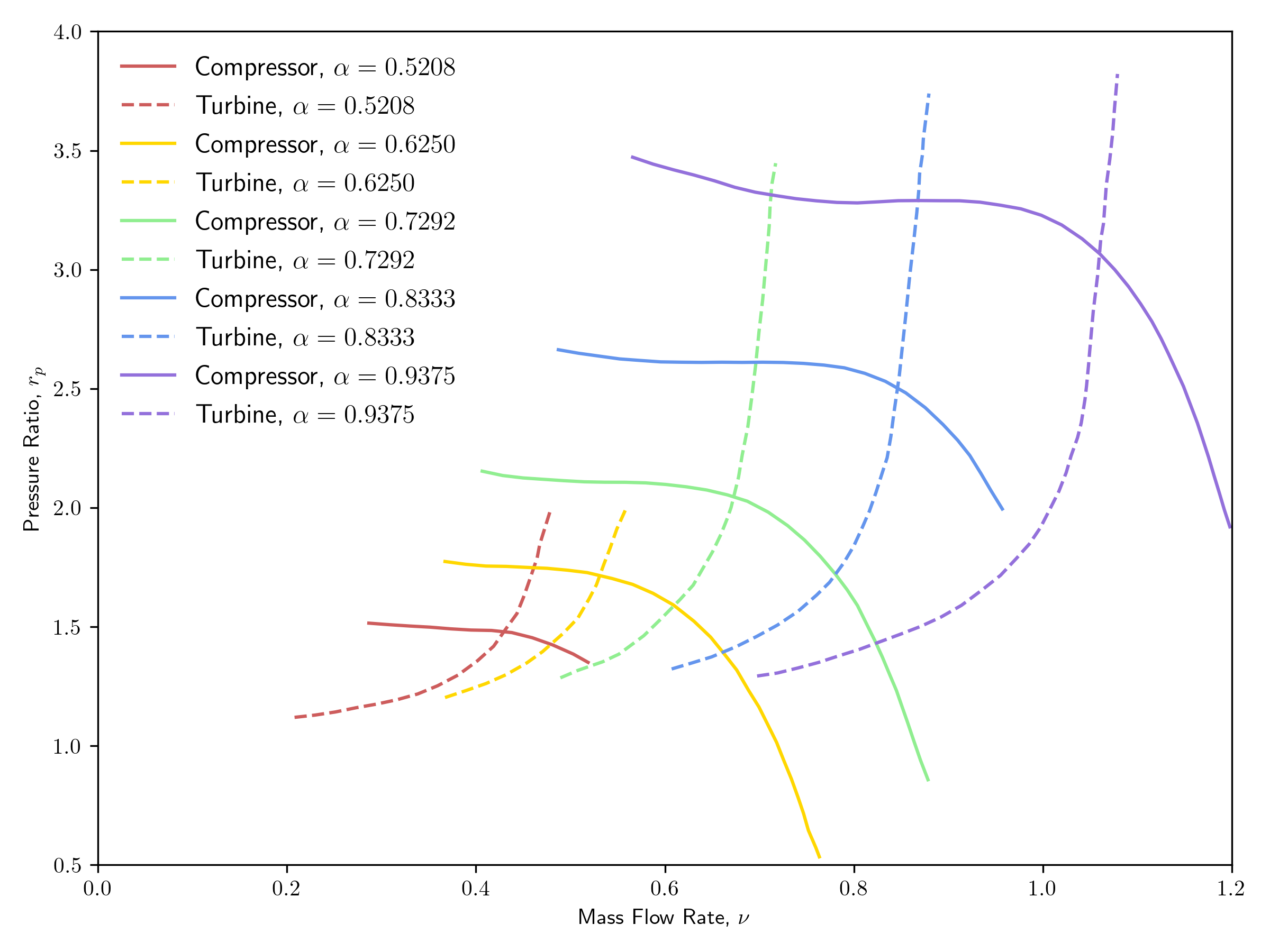
Figure 1: Pressure ratio curves for the compressor and turbine.
The efficiencies of both the compressor and turbine were set to constant values.
Finally, a generator is modeled using a ShaftConnectedMotor by using a negative torque of the form
where is a positive value. This is accomplished as follows:
[Components<<<{"href": "../../../../syntax/Components/index.html"}>>>]
  [generator]
    type = ShaftConnectedMotor<<<{"description": "Motor to drive a shaft component", "href": "../../../../source/components/ShaftConnectedMotor.html"}>>>
    inertia<<<{"description": "Moment of inertia from the motor [N-m]"}>>> = ${I_generator}
    torque<<<{"description": "Driving torque supplied by the motor [kg-m^2]"}>>> = generator_torque_fn
  []
[]
with the following function:
[Functions<<<{"href": "../../../../syntax/Functions/index.html"}>>>]
  [generator_torque_fn]
    type = ParsedFunction<<<{"description": "Function created by parsing a string", "href": "../../../../source/functions/MooseParsedFunction.html"}>>>
    expression<<<{"description": "The user defined function."}>>> = 'slope * t'
    symbol_names<<<{"description": "Symbols (excluding t,x,y,z) that are bound to the values provided by the corresponding items in the symbol_values vector."}>>> = 'slope'
    symbol_values<<<{"description": "Constant numeric values, postprocessor names, function names, and scalar variables corresponding to the symbols in symbol_names."}>>> = '${generator_torque_per_shaft_speed}'
  []
[]
Closed Brayton Cycle
The model discussed in this section can be found in the following input file: closed_brayton_cycle.i.
In the closed cycle, a strong convection source term is applied to bring the working fluid back to near the ambient temperature:
[Components<<<{"href": "../../../../syntax/Components/index.html"}>>>]
  [cooling]
    type = HeatTransferFromSpecifiedTemperature1Phase<<<{"description": "Heat transfer connection from a fixed temperature function for 1-phase flow", "href": "../../../../source/components/HeatTransferFromSpecifiedTemperature1Phase.html"}>>>
    flow_channel<<<{"description": "Name of flow channel component to connect to"}>>> = pipe6
    T_wall<<<{"description": "Specified wall temperature [K]"}>>> = ${T_cold}
    Hw<<<{"description": "Convective heat transfer coefficient [W/(m^2-K)]"}>>> = htc_wall_fn
  []
[]
Open Brayton Cycle
The model discussed in this section can be found in the following input file: open_brayton_cycle.i.
In the open cycle, instead of a heat sink, there is an inlet connected to the compressor inlet piping, and an outlet connected to the turbine outlet piping. For the inlet, the stagnation pressure and temperature formulation is appropriate, since the environment can be approximated to be at rest. The ambient pressure and temperature can then be used for and , respectively:
[Components<<<{"href": "../../../../syntax/Components/index.html"}>>>]
  [inlet]
    type = InletStagnationPressureTemperature1Phase<<<{"description": "Boundary condition with prescribed stagnation pressure and temperature for 1-phase flow channels.", "href": "../../../../source/components/InletStagnationPressureTemperature1Phase.html"}>>>
    input<<<{"description": "Name of the input"}>>> = 'pipe1:in'
    p0<<<{"description": "Prescribed stagnation pressure [Pa]"}>>> = ${p_ambient}
    T0<<<{"description": "Prescribed stagnation temperature [K]"}>>> = ${T_ambient}
  []
[]
There is a single outlet formulation, which specifies the ambient pressure:
[Components<<<{"href": "../../../../syntax/Components/index.html"}>>>]
  [outlet]
    type = Outlet1Phase<<<{"description": "Boundary condition with prescribed pressure for 1-phase flow channels.", "href": "../../../../source/components/Outlet1Phase.html"}>>>
    input<<<{"description": "Name of the input"}>>> = 'pipe5:out'
    p<<<{"description": "Prescribed pressure [Pa]"}>>> = ${p_ambient}
  []
[]
Results
Figure 2 and Figure 3 show the shaft speed transient for the open and closed cycles, respectively. The shaft speed profile indicates that the motor torque is fairly dominant in this example, as the profile appears to be an integral of the motor torque profile that was used; the motor torque was ramped up from zero to a max at and then back down to zero at . The profile seen here may not necessarily be realistic, for several reasons, including the following:
Moments of inertia of the various shaft components were chosen arbitrarily,
The motor torque profile was chosen arbitrarily,
The generator torque relationship was chosen arbitrarily, and
Friction losses on the shaft were omitted.

Figure 2: Shaft speed transient for the open cycle.
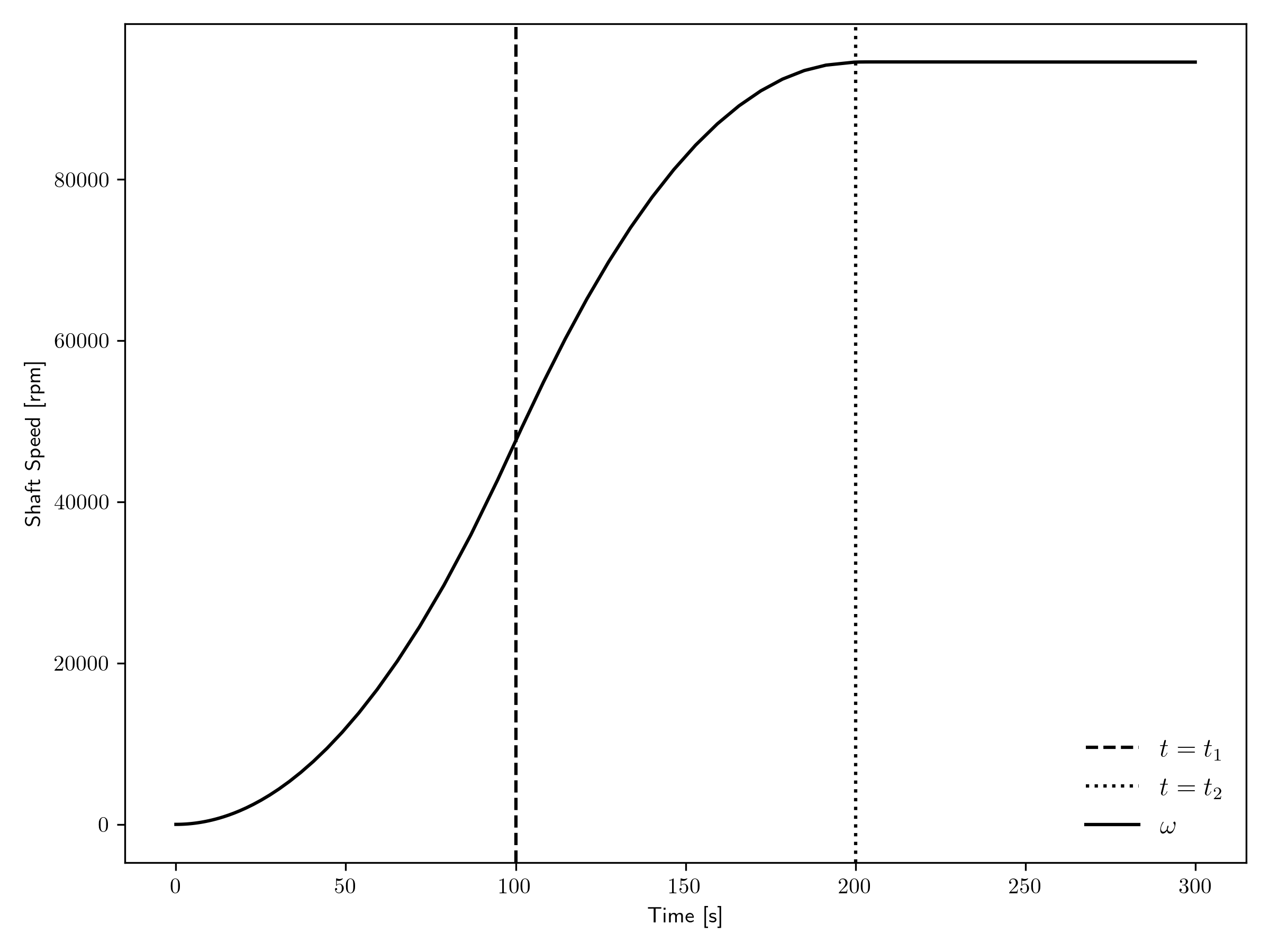
Figure 3: Shaft speed transient for the closed cycle.
Figure 4 and Figure 5 show the mass flow rate transient for the open and closed cycles, respectively. At the beginning of the transient, the mass flow rate is zero, and as the shaft starts spinning, either the compressor or turbine first gets a pressure ratio greater than 1, which allows flow to begin. It can be seen that the mass flow rate is actually slightly negative before the compressor finally activates. Then as the pressure ratios further increase, the mass flow rate increases until it reaches the steady condition.
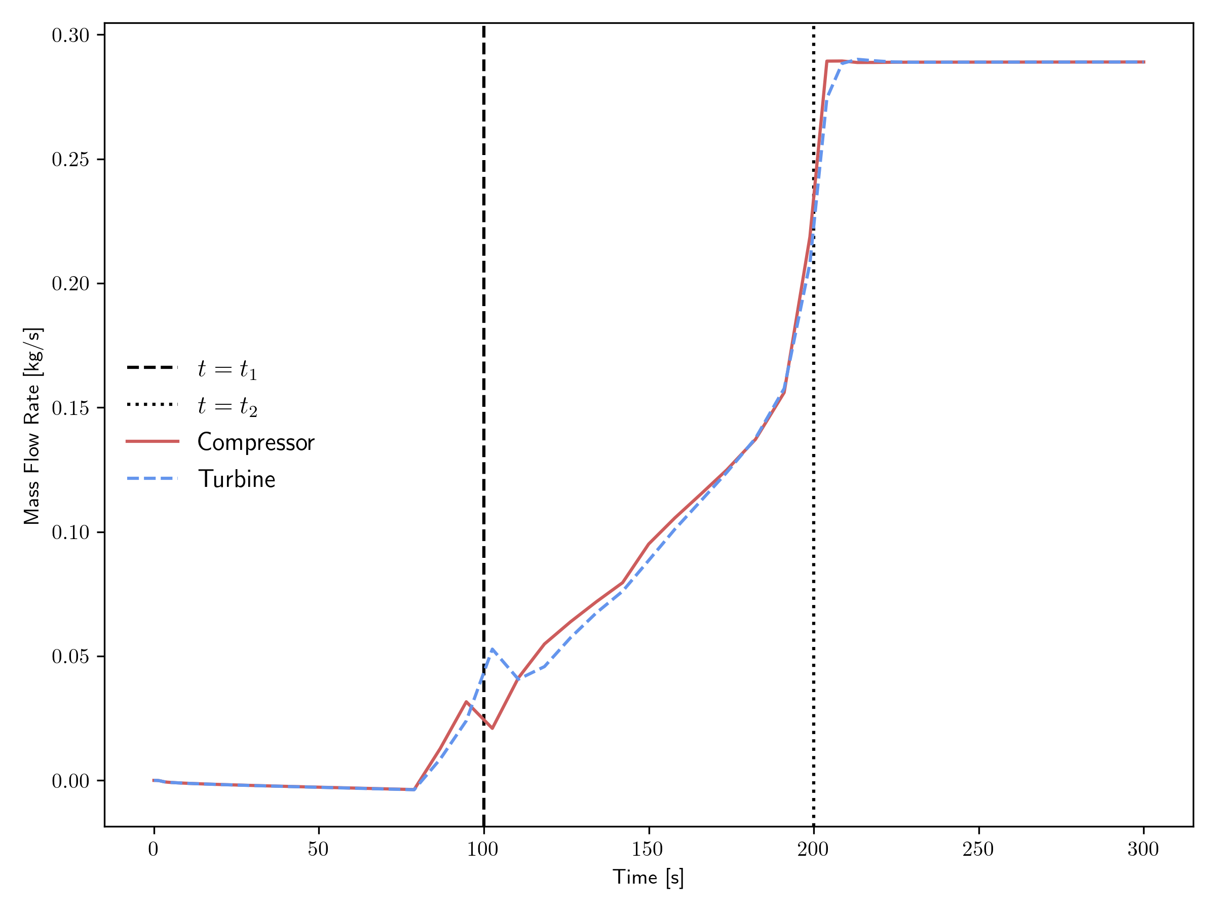
Figure 4: Mass flow rate transient for the open cycle.
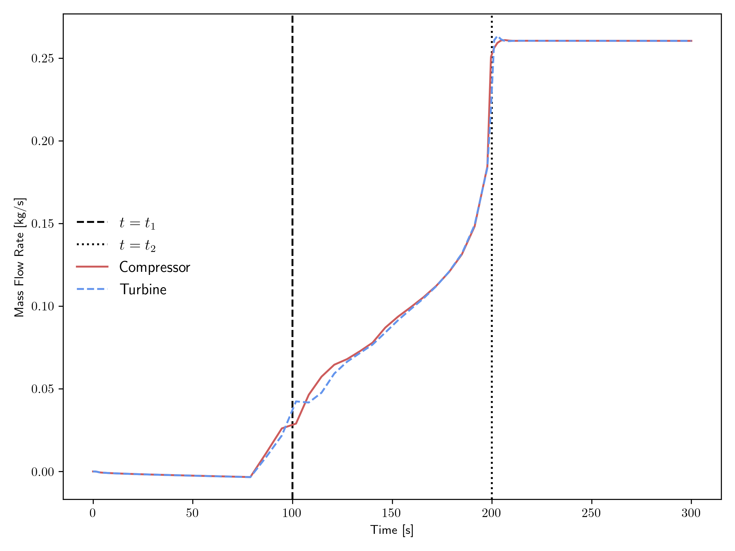
Figure 5: Mass flow rate transient for the closed cycle.
Figure 6 and Figure 7 show the pressure ratio transient for the open and closed cycles, respectively. Recall that this example starts with everything at rest, i.e., there is initially no flow or shaft speed. The motor ramps up the shaft speed to get the compressor working, but only around s does the pressure ratio of the compressor and turbine start to exceed 1, which is the point at which flow can start to develop.
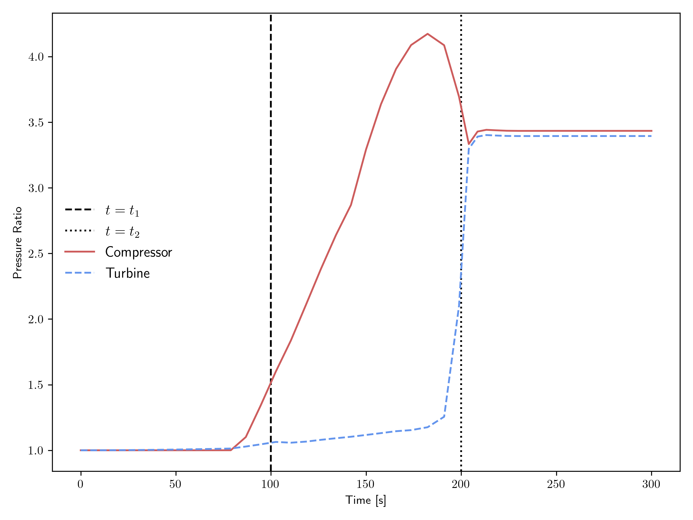
Figure 6: Pressure ratio transient for the open cycle.
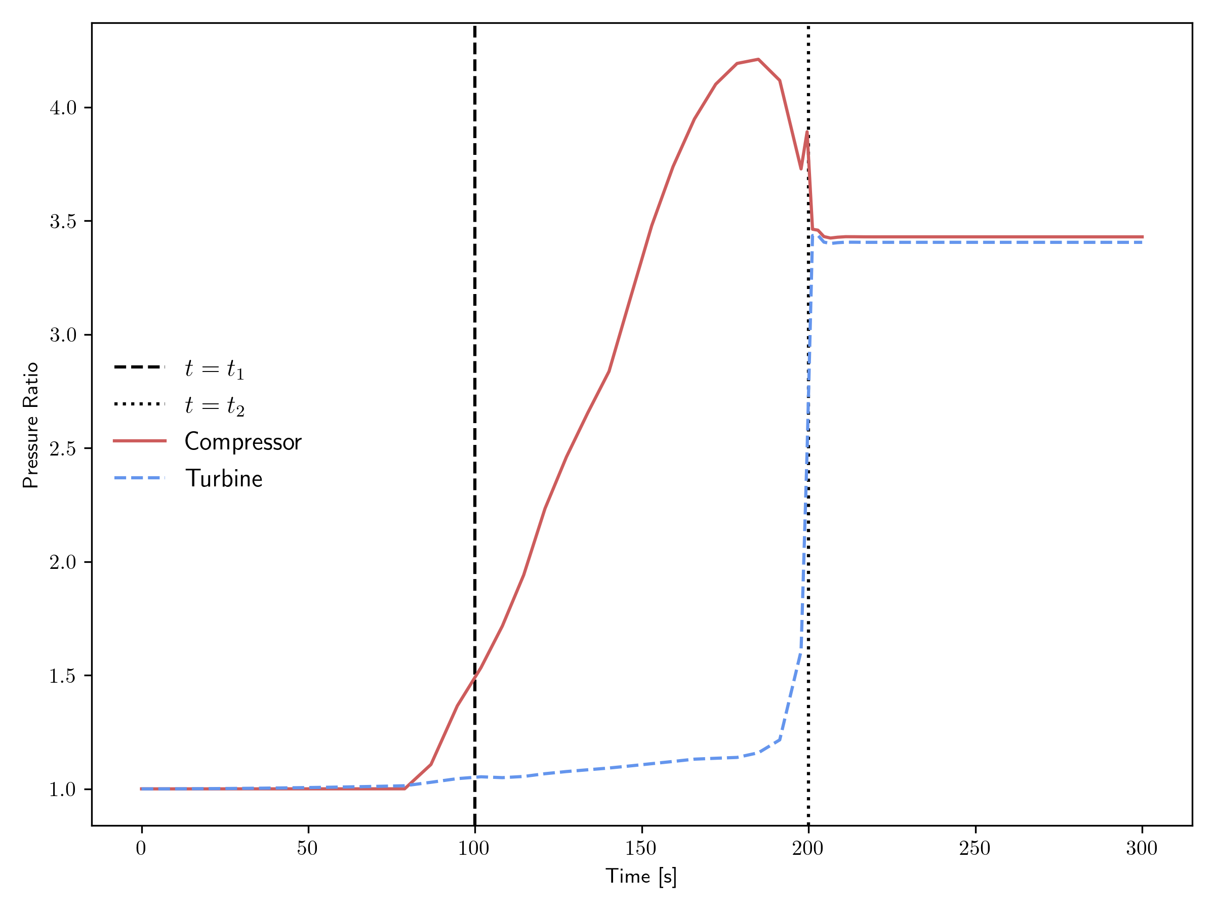
Figure 7: Pressure ratio transient for the closed cycle.
Figure 8 and Figure 9 show the power transient for the open and closed cycles, respectively. Several quantities are included on these plots:
, the thermal power provided by the heat source,
, the thermal power provided by the heat sink (closed cycle only),
, the power taken by the generator (and thus becomes useful electrical power),
, the power consumed by the compressor, and
, the power provided by the turbine.
Not shown in these plots is the power consumed by the motor, as it dwarfs the other powers shown for the period of the transient where it is most active. In a practical setup, the motor power may be much less and just operates for a much longer period during startup.
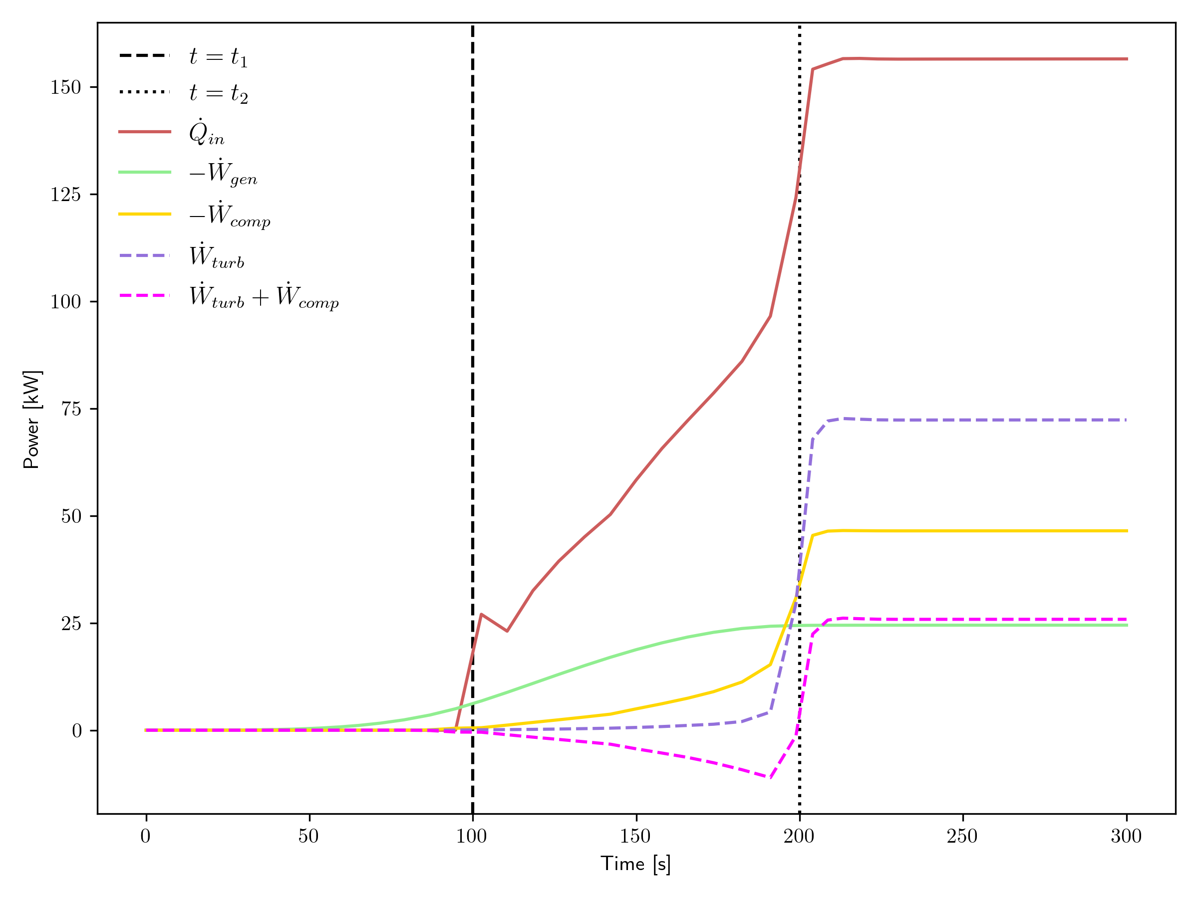
Figure 8: Power transient for the open cycle.
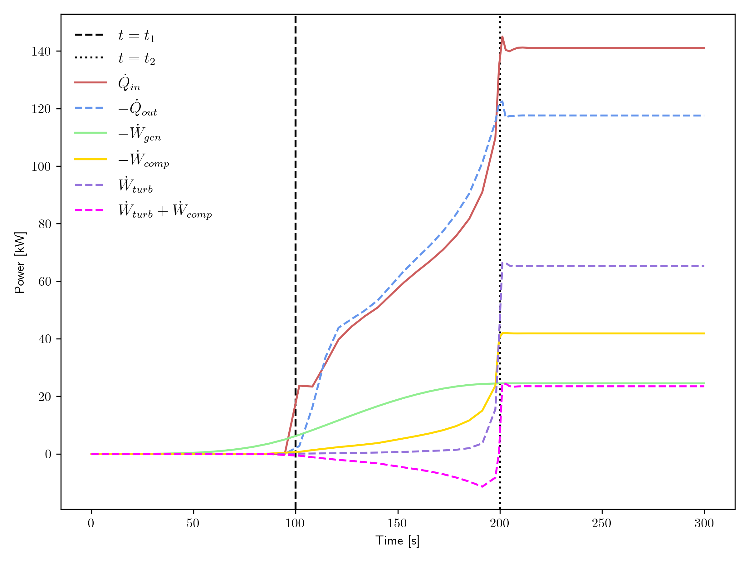
Figure 9: Power transient for the closed cycle.
Comparing the various plots between the open and closed cycles supports the assertion that a closed Brayton cycle approximation can yield very similar results to an open Brayton cycle.
References
- Donna Post Guillen and Daniel S. Wendt.
Integration of a microturbine power conversion unit in MAGNET.
Technical Report INL/EXT-20-57712, Idaho National Laboratory, 8 2020.
URL: https://www.osti.gov/biblio/1736010, doi:10.2172/1736010.[Export]