SOBOL Sensitivity Analysis
The following example converts Parameter Study to perform a global variance-based sensitivity analysis following the method of Saltelli (2002).
Input File
To perform a the sensitivity analysis only two minor changes to the input file from Parameter Study need to occur: the sampler needs be changed and another statistics calculation object needs to be added, the remainder of the file remains the same. The exception being that the sampler name in a few of the objects was updated to use the "sobol" Sampler name, as defined in the following sub-section.
Sobol Sampler
The Sobol sampling scheme consists of using a sample and re-sample matrix to create a series of matrices that can be used to compute first-order, second-order, and total-effect sensitivity indices. The first-order indices are the portion of the variance in the quantity of interest (e.g., ) due to the variance of the uncertain parameters (e.g., ). The second-order indices are the portion of the variance in the quantity of interest due to the variance two uncertain parameters interacting (e.g., as ). Finally, the total-effect indices are the portion of the variance of the quantity of interest due to the variance of an uncertain parameter and all interactions with the other parameters. For complete details of the method please refer to Saltelli (2002).
The Sobol object requires two input samplers to form the sample and re-sample matrix. Thus, the Samplers block contains three sample objects. The first two are used by the third, the "sobol" sampler, which is the Sampler used by the other objects in the simulation.
[Samplers<<<{"href": "../../../syntax/Samplers/index.html"}>>>]
  [hypercube_a]
    type = LatinHypercube<<<{"description": "Latin Hypercube Sampler.", "href": "../../../source/samplers/LatinHypercubeSampler.html"}>>>
    num_rows<<<{"description": "The size of the square matrix to generate."}>>> = 10000
    distributions<<<{"description": "The distribution names to be sampled, the number of distributions provided defines the number of columns per matrix."}>>> = 'gamma q_0 T_0 s'
    seed<<<{"description": "Random number generator initial seed"}>>> = 2011
  []
  [hypercube_b]
    type = LatinHypercube<<<{"description": "Latin Hypercube Sampler.", "href": "../../../source/samplers/LatinHypercubeSampler.html"}>>>
    num_rows<<<{"description": "The size of the square matrix to generate."}>>> = 10000
    distributions<<<{"description": "The distribution names to be sampled, the number of distributions provided defines the number of columns per matrix."}>>> = 'gamma q_0 T_0 s'
    seed<<<{"description": "Random number generator initial seed"}>>> = 2013
  []
  [sobol]
    type = Sobol<<<{"description": "Sobol variance-based sensitivity analysis Sampler.", "href": "../../../source/samplers/SobolSampler.html"}>>>
    sampler_a<<<{"description": "The 'sample' matrix."}>>> = hypercube_a
    sampler_b<<<{"description": "The 're-sample' matrix."}>>> = hypercube_b
  []
[]The sobol method implemented here requires model evaluations, where is the number of uncertain parameters (4) and is the number of replicates (10,000). Therefore, for this example 100,000 model evaluations were performed to compute the indices.
Sobol Statistics
The values of the first-order, second-order, and total-effect are computed by the SobolReporter object. This object is a Reporter, as such it is added to the Reporters block. The output of the object includes all the indices for each of the vectors supplied.
[Reporters<<<{"href": "../../../syntax/Reporters/index.html"}>>>]
  [results]
    type = StochasticReporter<<<{"description": "Storage container for stochastic simulation results coming from Reporters.", "href": "../../../source/reporters/StochasticReporter.html"}>>>
    outputs<<<{"description": "Vector of output names where you would like to restrict the output of variables(s) associated with this object"}>>> = none
  []
  [stats]
    type = StatisticsReporter<<<{"description": "Compute statistical values of a given VectorPostprocessor objects and vectors.", "href": "../../../source/reporters/StatisticsReporter.html"}>>>
    reporters<<<{"description": "List of Reporter values to utilized for statistic computations."}>>> = 'results/results:T_avg:value results/results:q_left:value'
    compute<<<{"description": "The statistic(s) to compute for each of the supplied vector postprocessors."}>>> = 'mean'
    ci_method<<<{"description": "The method to use for computing confidence level intervals."}>>> = 'percentile'
    ci_levels<<<{"description": "A vector of confidence levels to consider, values must be in (0, 1)."}>>> = '0.05 0.95'
  []
  [sobol]
    type = SobolReporter<<<{"description": "Compute SOBOL statistics values of a given VectorPostprocessor or Reporter objects and vectors.", "href": "../../../source/reporters/SobolReporter.html"}>>>
    sampler<<<{"description": "SobolSampler object."}>>> = sobol
    reporters<<<{"description": "List of Reporter values to utilized for statistic computations."}>>> = 'results/results:T_avg:value results/results:q_left:value'
    ci_levels<<<{"description": "A vector of confidence levels to consider, values must be in (0, 1)."}>>> = '0.05 0.95'
  []
[]Results
If JSON output is enabled, the SobolReporter object will write a file that contains columns of data. Each column comprises of the computed indices for the quantities of interest. For example, Listing 1 is and example output from the SobolReporter object for this example problem.
Listing 1: Computed Sobol indices for the example heat conduction problem.
{
"reporters": {
"sobol": {
"confidence_intervals": {
"levels": [
0.05,
0.95
],
"method": "percentile",
"replicates": 10000,
"seed": 1
},
"indices": [
"FIRST_ORDER",
"TOTAL",
"SECOND_ORDER"
],
"num_params": 4,
"type": "SobolReporter",
"values": {
"results_results:T_avg:value": {
"type": "SobolIndices<double>"
},
"results_results:q_left:value": {
"type": "SobolIndices<double>"
}
}
},
"stats": {
"confidence_intervals": {
"levels": [
0.05,
0.95
],
"method": "percentile",
"replicates": 10000,
"seed": 1
},
"type": "StatisticsReporter",
"values": {
"results_results:T_avg:value_MEAN": {
"stat": "MEAN",
"type": "std::pair<double, std::vector<double>>"
},
"results_results:q_left:value_MEAN": {
"stat": "MEAN",
"type": "std::pair<double, std::vector<double>>"
}
}
}
},
"time_steps": [
{
"sobol": {
"results_results:T_avg:value": {
"FIRST_ORDER": [
[
2.1263340395510633,
-0.1704186766506682,
0.8910628142531882,
1.3282033876672334
],
[
[
-1.9245992759047956,
-0.14744423678401847,
-0.7405474538071208,
-1.0243646808232845
],
[
1.6905363618407854,
0.1450721789342176,
0.7404629509699922,
1.0489650198653504
]
]
],
"SECOND_ORDER": [
[
[
2.1263340395510633,
-1.5858228336921647,
-2.3644853561144674,
-2.579482734445585
],
[
-1.5858228336921647,
-0.1704186766506682,
-0.4523042536164599,
-0.367641436024306
],
[
-2.3644853561144674,
-0.4523042536164599,
0.8910628142531882,
-1.5711186359853193
],
[
-2.579482734445585,
-0.367641436024306,
-1.5711186359853193,
1.3282033876672334
]
],
[
[
[
-1.9245992759047956,
-2.4218500787437396,
-3.617008106448411,
-5.862519943209779
],
[
-2.4218500787437396,
-0.14744423678401847,
-0.832270330827527,
-2.8610595323068497
],
[
-3.617008106448411,
-0.832270330827527,
-0.7405474538071208,
-3.5757491943596618
],
[
-5.862519943209779,
-2.8610595323068497,
-3.5757491943596618,
-1.0243646808232845
]
],
[
[
1.6905363618407854,
3.1470133995628062,
4.514567212267766,
6.89107489125814
],
[
3.1470133995628062,
0.1450721789342176,
1.0571317999622678,
4.298526262974558
],
[
4.514567212267766,
1.0571317999622678,
0.7404629509699922,
4.456668649214556
],
[
6.89107489125814,
4.298526262974558,
4.456668649214556,
1.0489650198653504
]
]
]
],
"TOTAL": [
[
0.6716920085825218,
0.42122423634195616,
0.3537665831825715,
0.7240444008318918
],
[
[
-0.418787576163522,
-1.0914201016146587,
-1.461531958201411,
-0.05300938717236381
],
[
2.34661879291093,
2.6160736708372916,
3.0599292054684,
1.7735775267008993
]
]
]
},
"results_results:q_left:value": {
"FIRST_ORDER": [
[
1.8235469621932516,
0.06461083007807501,
0.49024479333618587,
0.019712160157117343
],
[
[
-4.271886175566092,
-0.21358955122248832,
-1.1140788037385907,
-0.13405082544978414
],
[
3.742866431612808,
0.2143580106124228,
1.044098143434037,
0.11379671226869181
]
]
],
"SECOND_ORDER": [
[
[
1.8235469621932516,
-1.3905505375487972,
-1.468198101809389,
-1.375093249672925
],
[
-1.3905505375487972,
0.06461083007807501,
-0.12126951652702196,
-0.047038385516822184
],
[
-1.468198101809389,
-0.12126951652702196,
0.49024479333618587,
-0.2655312466346423
],
[
-1.375093249672925,
-0.047038385516822184,
-0.2655312466346423,
0.019712160157117343
]
],
[
[
[
-4.271886175566092,
-5.304910750107738,
-7.760475751994446,
-5.214012530917785
],
[
-5.304910750107738,
-0.21358955122248832,
-2.249348007191563,
-0.39487323449307704
],
[
-7.760475751994446,
-2.249348007191563,
-1.1140788037385907,
-1.8734667070660467
],
[
-5.214012530917785,
-0.39487323449307704,
-1.8734667070660467,
-0.13405082544978414
]
],
[
[
3.742866431612808,
6.469542112008098,
8.967736860567939,
6.0827138324513825
],
[
6.469542112008098,
0.2143580106124228,
3.3271039032372682,
0.5153962553256152
],
[
8.967736860567939,
3.3271039032372682,
1.044098143434037,
2.0634135974545433
],
[
6.0827138324513825,
0.5153962553256152,
2.0634135974545433,
0.11379671226869181
]
]
]
],
"TOTAL": [
[
0.8361004068731036,
0.3945056560029335,
0.346048550986653,
0.45400871228396333
],
[
[
0.05818944660486691,
-1.878159764251841,
-2.3161866666666224,
-1.3652499049416096
],
[
1.7554390551839805,
3.5022906001104546,
3.853777814700177,
2.8919833475141856
]
]
]
}
},
"stats": {
"results_results:T_avg:value_MEAN": [
202.8201819567622,
[
194.29058053592289,
211.62739771551531
]
],
"results_results:q_left:value_MEAN": [
182.62967983344282,
[
169.07983812958125,
196.41814128692013
]
]
},
"time": 2.0,
"time_step": 2
}
]
}
For each set of indices (FIRST_ORDER, SECOND_ORDER, and TOTAL) contains a pair entries: the first is the values computed and the second corresponds to the 5% and 95% confidence intervals. This problem examines four uncertain parameters, so each element of the set of indices corresponds to the parameter indicated in the input file (, , , and ). See SobolReporter for further information regarding the output.
For the problem at hand, the first-order and second-order indices for the two quantities of interest are presented in Table 1 and Table 2. The diagonal entries are the first-order indices and the off-diagonal terms are the second-order indices. For example for the first order-index for is and the second-order index for interacting with . The negative values are essentially zero, if more replicates were executed these numbers would become closer to zero.
python ../../python/moose_stochastic_tools/visualize_sobol.py main_out.json  --markdown-table \
--values results_results:T_avg:value --stat second_order \
--param-names '$\gamma$' '$q_0$' '$T_0$' '$s$' \
--number-format .3g
Table 1: First-order and second-order Sobol indices for .
| (5.0%, 95.0%) CI | ||||
|---|---|---|---|---|
| 0.687 (0.625, 0.765) | - | - | - | |
| 0.0138 (-0.11, 0.138) | 0.00735 (0.00595, 0.00887) | - | - | |
| 0.0212 (-0.115, 0.159) | -0.000649 (-0.00788, 0.00631) | 0.0898 (0.0803, 0.101) | - | |
| 0.0111 (-0.147, 0.171) | -0.00372 (-0.0183, 0.0107) | -0.00414 (-0.0285, 0.0203) | 0.206 (0.186, 0.231) |
python ../../python/moose_stochastic_tools/visualize_sobol.py main_out.json  --markdown-table \
--values results_results:q_left:value --stat second_order \
--param-names '$\gamma$' '$q_0$' '$T_0$' '$s$' \
--number-format .3g
Table 2: First-order and second-order Sobol indices for .
| (5.0%, 95.0%) CI | ||||
|---|---|---|---|---|
| 0.822 (0.771, 0.88) | - | - | - | |
| 0.00132 (-0.1, 0.104) | 0.0286 (0.0262, 0.0312) | - | - | |
| 0.00552 (-0.108, 0.12) | -0.00308 (-0.00887, 0.00257) | 0.134 (0.125, 0.145) | - | |
| 7.92e-05 (-0.0992, 0.1) | -0.00201 (-0.00447, 0.000333) | -0.000977 (-0.00868, 0.00665) | 0.0049 (0.0038, 0.0061) |
The data in these two tables clearly indicates that a majority of the variance of both quantities of interest are due to the variance of , also affects and affects . Additionally, a small contribution of the variance is from a second-order interaction, , between and . The importance of , , and is further evident by the total-effect indices, as shown in Table 3.
python ../../python/moose_stochastic_tools/visualize_sobol.py main_out.json --markdown-table --stat total \
--names '{"results_results:T_avg:value":"$T_{avg}$", "results_results:q_left:value":"$q_{left}$"}' \
--param-names '$\gamma$' '$q_0$' '$T_0$' '$s$' \
--number-format .3g
Table 3: Total-effect Sobol indices for and .
| (5.0%, 95.0%) CI | ||||
|---|---|---|---|---|
| 0.699 (0.665, 0.728) | 0.0131 (-0.0955, 0.102) | 0.108 (0.00979, 0.189) | 0.208 (0.121, 0.28) | |
| 0.836 (0.823, 0.846) | 0.0406 (-0.0249, 0.0979) | 0.158 (0.0999, 0.208) | 0.0149 (-0.0517, 0.0736) |
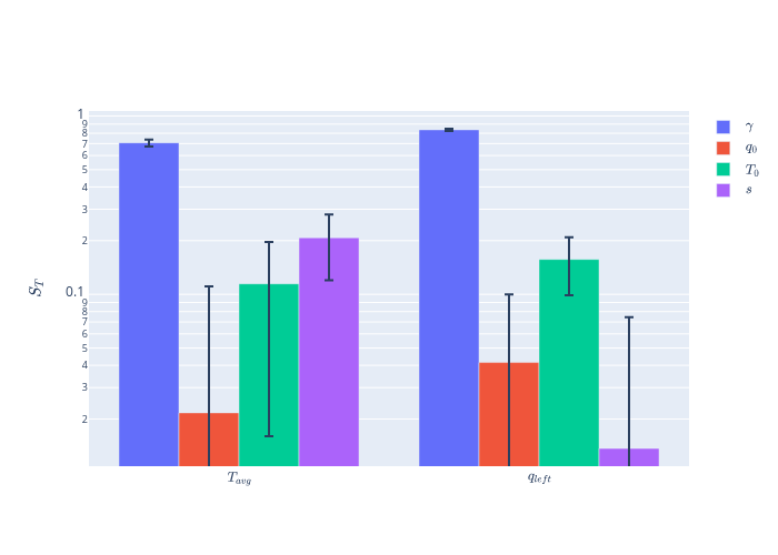
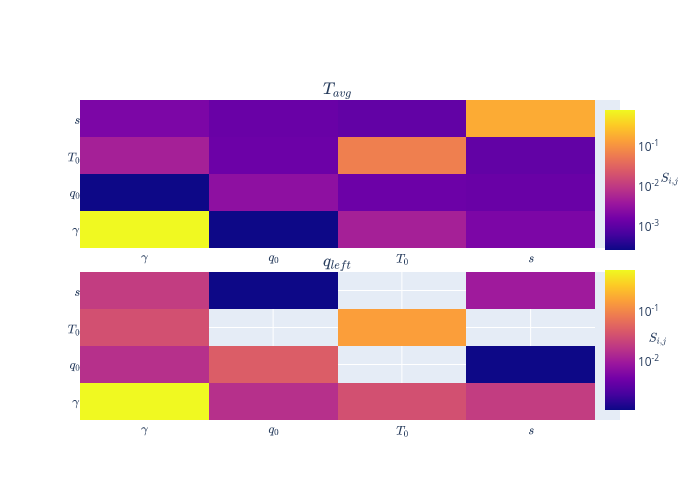
To help visualize the sensitivities, visualize_sobol.py can also represent it as a bar pot or heat map:
python ../../python/moose_stochastic_tools/visualize_sobol.py main_out.json --bar-plot --log-scale --stat total \
--names '{"results_results:T_avg:value":"$T_{avg}$", "results_results:q_left:value":"$q_{left}$"}' \
--param-names '$\gamma$' '$q_0$' '$T_0$' '$s$'
python ../../python/moose_stochastic_tools/visualize_sobol.py main_out.json --heatmap --log-scale --stat second_order \
--names '{"results_results:T_avg:value":"$T_{avg}$", "results_results:q_left:value":"$q_{left}$"}' \
--param-names '$\gamma$' '$q_0$' '$T_0$' '$s$'
References
- Andrea Saltelli.
Making best use of model evaluations to compute sensitivity indices.
Computer Physics Communications, 145(2):280–297, 2002.
URL: https://doi.org/10.1016/S0010-4655(02)00280-1.[Export]