Parameter Study

A parameter study is defined here as performing a simulation with varying uncertain parameters and computing quantities of interest for each set of uncertain parameters. This example is a more detailed example of what is presented in Monte Carlo Example, which is also a parameter study.

Problem Statement

To demonstrate how to perform a parameter study the transient heat equation will be used.

\frac{\partial T}{\partial t} - \nabla\cdot\gamma\nabla T + s = 0,

where $T$ is temperature, $t$ is time, $\gamma$ is diffusivity, and $s$ is a heat source term. This problem shall be solved on a 2D unit square domain. The left side is subjected to a Dirichlet condition $T=T_0$ . The right side of the domain is subject to a Neumann condition $-\gamma\nabla T \cdot \hat{n} = q_0$ , where $\hat{n}$ is the outward facing normal vector from the boundary.

The boundary conditions $T_0$ and $q_0$ as well as the diffusivity ( $\gamma$ ) and the source term $s$ are assumed to be known. However, these parameters have some associated uncertainty. The effect of the uncertainty on the average temperature and heat flux on the left boundary after one second of simulation time is desired, defined as $T_{avg} = \bar{T}(t=1)$ and $q_{left} = q(t=1,x=0)$ .

Heat Equation Problem

The first step in performing a parameter study is to create an input file that solves your problem without uncertain parameters. For the example problem this will be done assuming $\gamma=1$ , $s=100$ , $T_0=300$ , and $q_0=-100$ .

The complete input file for this problem is provided in Listing 1. The only item that is atypical from a MOOSE simulation input file is the existence of the Controls block, which here simply creates a SamplerReceiver object. This block is required for the parameter study, but shall be discussed in the Transfers Block section.

Listing 1: Complete input file for example heat equation problem to be used in parameter study.

[Mesh]
  type = GeneratedMesh
  dim = 2
  nx = 10
  ny = 10
[]

[Variables/T]
  initial_condition = 300
[]

[Kernels]
  [time]
    type = ADTimeDerivative
    variable = T
  []
  [diff]
    type = ADMatDiffusion
    variable = T
    diffusivity = diffusivity
  []
  [source]
    type = ADBodyForce
    variable = T
    value = 100
    function = 1
  []
[]

[BCs]
  [left]
    type = ADDirichletBC
    variable = T
    boundary = left
    value = 300
  []
  [right]
    type = ADNeumannBC
    variable = T
    boundary = right
    value = -100
  []
[]

[Materials/constant]
  type = ADGenericConstantMaterial
  prop_names = 'diffusivity'
  prop_values = 1
[]

[Executioner]
  type = Transient
  num_steps = 4
  dt = 0.25
[]

[Postprocessors]
  [T_avg]
    type = ElementAverageValue
    variable = T
    execute_on = 'initial timestep_end'
  []
  [q_left]
    type = ADSideDiffusiveFluxAverage
    variable = T
    boundary = left
    diffusivity = diffusivity
    execute_on = 'initial timestep_end'
  []
[]

[Controls/stochastic]
  type = SamplerReceiver
[]

[Outputs]
[]

Executing this file using the StochasticToolsApp can be done as follows

cd moose/modules/stochastic_tools/examples/parameter_study
../../stochastic_tools-opt -i diffusion.i

The simulation will perform four timesteps and should result in $T_{avg}=286$ and $q_{left}=1.73$ .

Main Input

To perform a parameter study an input file that will drive the stochastic simulations is required. This file will be referred to as the main input file and is responsible for defining the uncertain parameters, running the stochastic simulations, and collecting the stochastic results. The following sub-sections will step through each portion of the main file to explain the purpose. The complete analysis is discussed in Stochastic Results.

The specific parameter study performed in this tutorial can also done using the ParameterStudy syntax, shown in the code block below. However, it is very useful to learn each aspect of doing a stochastic simulation in the stochastic tools module, which is described in the following sub-sections.

Parameter study using ParameterStudy input block

[ParameterStudy]
  input = diffusion.i
  parameters = 'Materials/constant/prop_values Kernels/source/value BCs/right/value BCs/left/value'
  quantities_of_interest = 'T_avg/value q_left/value'

  sampling_type = lhs
  num_samples = 5000
  distributions = 'uniform weibull normal normal'
  uniform_lower_bound = 0.5
  uniform_upper_bound = 2.5
  weibull_location = -110
  weibull_scale = 20
  weibull_shape = 1
  normal_mean = '300 100'
  normal_standard_deviation = '45 25'
[]

StochasticTools Block

The StochasticTools block sets up the main file to be a driver for stochastic simulations but itself is not performing any sort of simulation. Setting up a main application without a simulation itself is the default behavior for this block, as such it is empty in this example.

[StochasticTools]
[]

Distributions and Samplers Blocks

The Distributions block defines the statistical distribution for each of the uncertain parameters ( $T_0$ , $q_0$ , $\gamma$ , and $s$ ) to be defined. For this example, the diffusivity ( $\gamma$ ) is defined by a uniform distribution, the flux ( $q_0$ ) by a three-parameter Weibull, and $T_0$ and $s$ a normal distribution.

[Distributions]
  [gamma]
    type = Uniform
    lower_bound = 0.5
    upper_bound = 2.5
  []
  [q_0]
    type = Weibull
    location = -110
    scale = 20
    shape = 1
  []
  [T_0]
    type = Normal
    mean = 300
    standard_deviation = 45
  []
  [s]
    type = Normal
    mean = 100
    standard_deviation = 25
  []
[]

The Samplers block defines how the distributions shall be sampled for the parameter study. In this case a Latin hypercube sampling strategy is employed. A total of 5000 samples are being used.

[Samplers]
  [hypercube]
    type = LatinHypercube
    num_rows = 5000
    distributions = 'gamma q_0 T_0 s'
  []
[]

For this problem the Sampler object is setup to run in "batch-restore" mode, which is a mode of operation for memory efficient creation of sub-applications. Please see Stochastic Tools Batch Mode for more information.

The input distributions for each of these four terms are included in Figure 1–Figure 4 for 5000 samples.

Figure 1: Input distribution of diffusivity ( $\gamma$ ).

Figure 2: Input distribution of flux boundary condition ( $q_0$ ).

Figure 3: Input distribution of temperature boundary condition ( $T_0$ ).

Figure 4: Input distribution of source term ( $s$ ).

Transfers Block

The Transfers block serves two purposes. First, the "parameters" sub-block instantiates a SamplerParameterTransfer object that transfers each row of data from the Sampler object to a sub-application simulation. Within the sub-application the parameters listed in this sub-block replace the values in the sub-application. This substitution occurs using the aforementioned SamplerReceiver object that exists in the Controls block of the sub-application input file. The receiver on the sub-application accepts the parameter names and values from the SamplerParameterTransfer object on the main application.

The "results" sub-block serves the second purpose by transferring the quantities of interest back to the main application. In this case those quantities are postprocessors on the sub-application that compute $T_{avg}$ and $q_{left}$ . These computed results are transferred from the sub-application to a StochasticReporter object (as discussed next).

[Transfers]
  [parameters]
    type = SamplerParameterTransfer
    to_multi_app = runner
    sampler = hypercube
    parameters = 'Materials/constant/prop_values Kernels/source/value BCs/right/value BCs/left/value'
  []
  [results]
    type = SamplerReporterTransfer
    from_multi_app = runner
    sampler = hypercube
    stochastic_reporter = results
    from_reporter = 'T_avg/value q_left/value'
  []
[]

Reporters Block

The Reporters block, as mentioned above, is used to collect the stochastic results. The "results" sub-block instantiates a StochasticReporter object, which is designed for this purpose. The resulting object will contain a vector for each of the quantities of interest: $T_{avg}$ and $q_{left}$ .

The StatisticsReporter object is designed to compute multiple statistics and confidence intervals for each of the input vectors. In this case it computes the mean and standard deviation for $T_{avg}$ and $q_{left}$ vectors in the "results" object as well as the 5% and 95% confidence level intervals. Please refer to the documentation for the StatisticsReporter object for further documentation and capabilities for this object.

[Reporters]
  [results]
    type = StochasticReporter
  []
  [stats]
    type = StatisticsReporter
    reporters = 'results/results:T_avg:value results/results:q_left:value'
    compute = 'mean stddev'
    ci_method = 'percentile'
    ci_levels = '0.05 0.95'
  []
[]

Outputs Block

The Outputs block enables the output of the Reporter data using JSON files, see JSON for more details.

[Outputs]
  execute_on = 'FINAL'
  [out]
    type = JSON
  []
[]

Stochastic Results

The input file described in the previous section can be run with the following command:

mpiexec -n <n> ../../stochastic_tools-opt -i main.i

The <n> is the number of processors to be run with. It is recommended to use a number greater than 8 to finish the calculation in a reasonable amount of time. The result will be an output of a main_out.json* file (one for each processor). If only one file is desired use the option Reporters/results/parallel_type=ROOT.

Quantity of Interest Distributions

The resulting distributions are for the quantities of interest: $T_{avg}$ and $q_{left}$ are presented in Figure 5 and Figure 6. These plots were generated using the following commands:

python ../../python/make_histogram.py main_out.json* -v results:T_avg:value --xlabel 'Average Temperature'
python ../../python/make_histogram.py main_out.json* -v results:q_left:value --xlabel 'Flux'

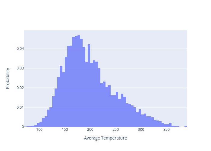
Figure 5: Resulting distribution of quantity of interest: $T_{avg}$ .

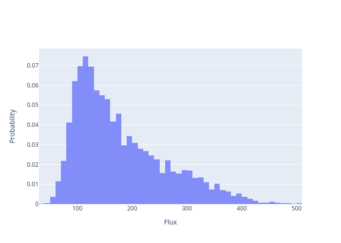
Figure 6: Resulting distribution of quantity of interest: $q_{left}$ .

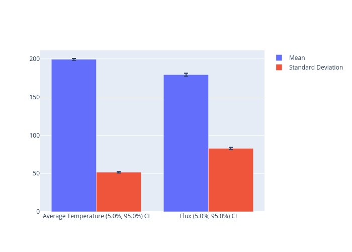
Statistics

Table 1 includes the computed statistics and confidence level intervals as computed by the StatisticsReporter object for the example heat conduction problem with 5000 samples. This table was generated in markdown format using the following command:

python ../../python/visualize_statistics.py main_out.json --markdown-table \
--names '{"results_results:T_avg:value":"$T_{avg}$","results_results:q_left:value":"$q_{left}$"}' \
--stat-names '{"MEAN":"Mean","STDDEV":"Standard Deviation"}'

Table 1:

Values	Mean	Standard Deviation
$T_{avg}$ (5.0%, 95.0%) CI	199.3 (198.1, 200.5)	51.55 (50.67, 52.41)
$q_{left}$ (5.0%, 95.0%) CI	179.3 (177.4, 181.2)	82.71 (81.24, 84.19)

These statistics can also be visualized with a bar plot:

python ../../python/visualize_statistics.py main_out.json --bar-plot \
--names '{"results_results:T_avg:value":"Average Temperature","results_results:q_left:value":"Flux"}' \
--stat-names '{"MEAN":"Mean","STDDEV":"Standard Deviation"}'

Time Dependent and Vector Quantities

Often, it is useful to perform parameter studies with quantities that are time-dependent. This section will show how to modify the previous inputs for quantities that are time-dependent or possibly vectors.

Sub-application Input Modifications

The only change to the sub-app input is the addition of a LineValueSampler vector-postprocessor that computes the spatial distribution of the temperature.

[VectorPostprocessors]
  [T_vec]
    type = LineValueSampler
    variable = T
    start_point = '0 0.5 0'
    end_point = '1 0.5 0'
    num_points = 11
    sort_by = x
    execute_on = 'initial timestep_end'
  []
[]

Main Input Modifications

The two significant modifications to the main input is the change to a SamplerTransientMultiApp and the addition of the Executioner block. The combination of these two blocks will run the sampled sub-applications in tandem with the time-step defined in the main input. The main application in this case will "drive" the overall simulation (and does support sub-cycling). Here, we use the same time stepping as in the sub-application.

[MultiApps]
  [runner]
    type = SamplerTransientMultiApp
    sampler = hypercube
    input_files = 'diffusion_time.i'
    mode = batch-restore
  []
[]

[Executioner]
  type = Transient
  num_steps = 4
  dt = 0.25
[]

We will also add the transfer for the LineValueSampler included in the sub input, while also computing statistics and transferring the x-coord values. Note that the ConstantReporter is just a place holder for the MultiAppReporterTransfer to transfer the x-coord data into.

[Transfers]
  [parameters]
    type = SamplerParameterTransfer
    to_multi_app = runner
    sampler = hypercube
    parameters = 'Materials/constant/prop_values Kernels/source/value BCs/right/value BCs/left/value'
  []
  [results]
    type = SamplerReporterTransfer
    from_multi_app = runner
    sampler = hypercube
    stochastic_reporter = results
    from_reporter = 'T_avg/value q_left/value T_vec/T'
  []
  [x_transfer]
    type = MultiAppReporterTransfer
    from_multi_app = runner
    subapp_index = 0
    from_reporters = T_vec/x
    to_reporters = const/x
  []
[]

[Reporters]
  [results]
    type = StochasticReporter
    outputs = none
  []
  [stats]
    type = StatisticsReporter
    reporters = 'results/results:T_avg:value results/results:q_left:value results/results:T_vec:T'
    compute = 'mean stddev'
    ci_method = 'percentile'
    ci_levels = '0.05 0.95'
  []
  [const]
    type = ConstantReporter
    real_vector_names = 'x'
    real_vector_values = '0'
  []
[]

Statistics

The output (main_time_out.json) will now have statistics for all three quantities for each time step. We can report this data using the following:

python ../../python/visualize_statistics.py main_time_out.json  --markdown-table \
--values results_results:T_avg:value results_results:q_left:value \
--names '{"results_results:T_avg:value":"Average Temperature","results_results:q_left:value":"Flux"}' \
--stats MEAN STDDEV --stat-names '{"MEAN":"Mean","STDDEV":"Standard Deviation"}'

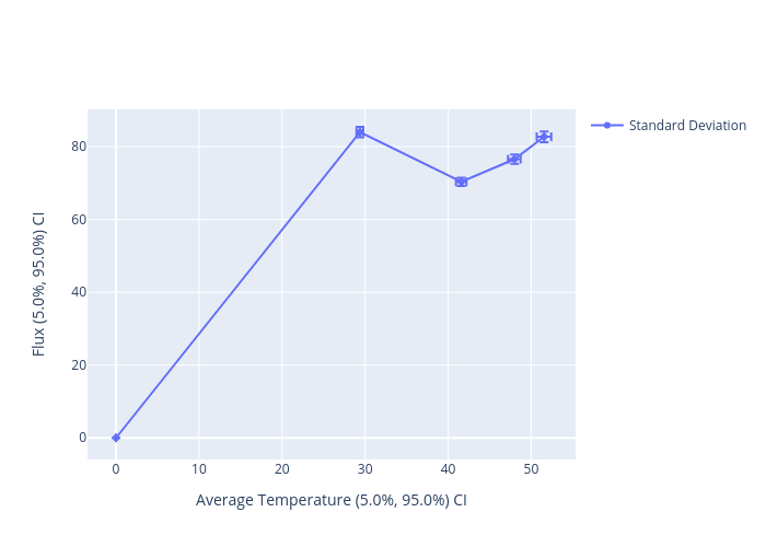
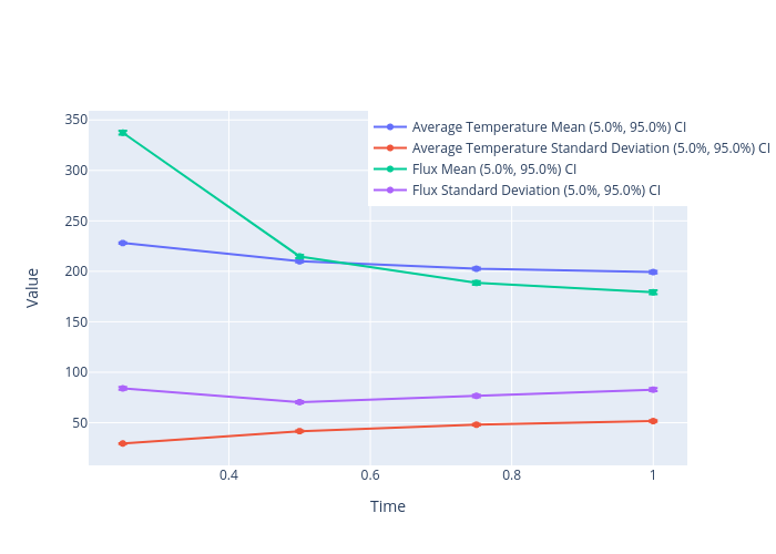
Values	Time	Mean	Standard Deviation
Average Temperature (5.0%, 95.0%) CI	0.25	228 (227.3, 228.7)	29.38 (28.96, 29.78)
	0.5	209.9 (209, 210.9)	41.58 (40.96, 42.19)
	0.75	202.5 (201.4, 203.7)	47.98 (47.21, 48.74)
	1	199.3 (198.1, 200.5)	51.55 (50.67, 52.41)
Flux (5.0%, 95.0%) CI	0.25	337.4 (335.4, 339.3)	84 (82.56, 85.43)
	0.5	214.8 (213.1, 216.4)	70.35 (69.23, 71.46)
	0.75	188.6 (186.8, 190.3)	76.56 (75.29, 77.82)
	1	179.3 (177.4, 181.2)	82.71 (81.24, 84.19)

python ../../python/visualize_statistics.py main_time_out.json --line-plot \
--values results_results:T_avg:value results_results:q_left:value \
--names '{"results_results:T_avg:value":"Average Temperature","results_results:q_left:value":"Flux"}' \
--stats MEAN STDDEV --stat-names '{"MEAN":"Mean","STDDEV":"Standard Deviation"}'

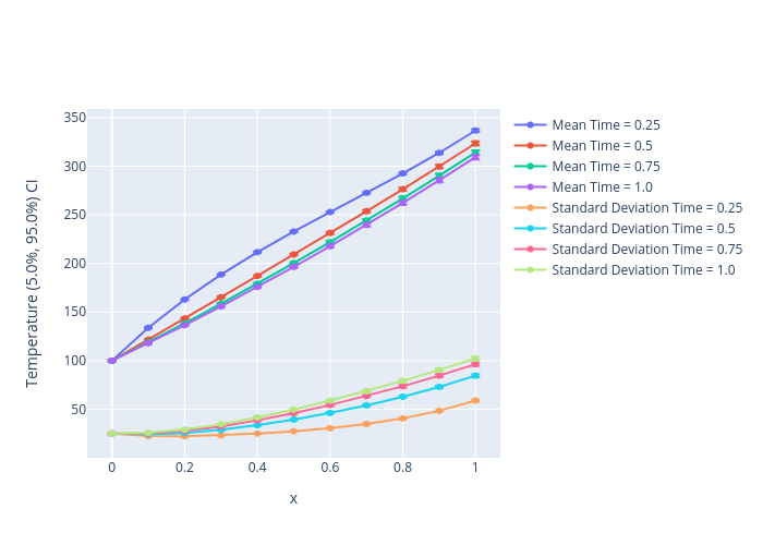
python ../../python/visualize_statistics.py main_time_out.json --line-plot \
--values results_results:T_vec:T --names '{"results_results:T_vec:T":"Temperature"}' \
--stats MEAN STDDEV --stat-names '{"MEAN":"Mean","STDDEV":"Standard Deviation"}' \
--xvalue x

Time Dependent Quantities with AccumulateReporter

You might find that using SamplerTransientMultiApp, like in the previous sections, is a bit restrictive. For instance, the time steps in the sub-app input must be defined by the steps in the main input. This restricts the use of TimeSteppers like IterationAdaptiveDT and sub-cycling sub-sub-apps becomes difficult. Also, SamplerTransientMultiApp does not support batch-reset mode, so there isn't a memory-efficient way of sampling with MultiAppSamplerControl.

An alternative to using SamplerTransientMultiApp is to leverage AccumulateReporter, which accumulates postprocessors/vector-postprocessor/reporters into vector where each element is the value at a certain time-step.

Sub-application Input Modifications

For this example, we will accumulate the T_avg and q_left postprocessors. We can accumulate T_vec from the previous section, but StatisticsReporter does not yet support vector-of-vector quantities.

[Reporters]
  [acc]
    type = AccumulateReporter
    reporters = 'T_avg/value q_left/value'
  []
[]

Main Input Modifications

There are no major modifications to the main input from the first section. We only need to replace the transferred values from *:value to acc:*:value.

[Transfers]
  [parameters]
    type = SamplerParameterTransfer
    to_multi_app = runner
    sampler = hypercube
    parameters = 'Materials/constant/prop_values Kernels/source/value BCs/right/value BCs/left/value'
  []
  [results]
    type = SamplerReporterTransfer
    from_multi_app = runner
    sampler = hypercube
    stochastic_reporter = results
    from_reporter = 'acc/T_avg:value acc/q_left:value'
  []
[]

[Reporters]
  [results]
    type = StochasticReporter
    outputs = none
  []
  [stats]
    type = StatisticsReporter
    reporters = 'results/results:acc:T_avg:value results/results:acc:q_left:value'
    compute = 'mean stddev'
    ci_method = 'percentile'
    ci_levels = '0.05 0.95'
  []
[]

Statistics

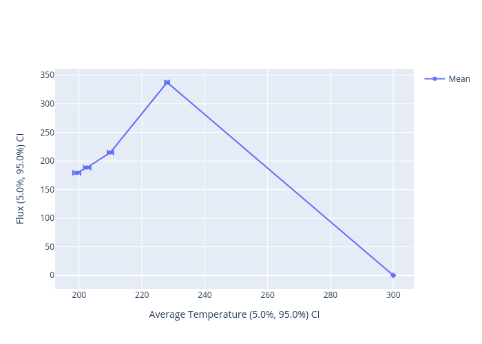
The output (main_vector_out.json) has the statistics for each quantity represented by a vector. All of the previous results can be reproduced with this output. One fancy thing we can do with this new output:

python ../../python/visualize_statistics.py main_vector_out.json --line-plot \
--names '{"results_results:acc:T_avg:value":"Average Temperature","results_results:acc:q_left:value":"Flux"}' \
--xvalue results_results:acc:T_avg:value \
--stats MEAN --stat-names '{"MEAN":"Mean"}'

python ../../python/visualize_statistics.py main_vector_out.json --line-plot \
--names '{"results_results:acc:T_avg:value":"Average Temperature","results_results:acc:q_left:value":"Flux"}' \
--xvalue results_results:acc:T_avg:value \
--stats STDDEV --stat-names '{"STDDEV":"Standard Deviation"}'

(contrib/moose/modules/stochastic_tools/examples/parameter_study/diffusion.i)

[Mesh]
  type = GeneratedMesh
  dim = 2
  nx = 10
  ny = 10
[]

[Variables/T]
  initial_condition = 300
[]

[Kernels]
  [time]
    type = ADTimeDerivative
    variable = T
  []
  [diff]
    type = ADMatDiffusion
    variable = T
    diffusivity = diffusivity
  []
  [source]
    type = ADBodyForce
    variable = T
    value = 100
    function = 1
  []
[]

[BCs]
  [left]
    type = ADDirichletBC
    variable = T
    boundary = left
    value = 300
  []
  [right]
    type = ADNeumannBC
    variable = T
    boundary = right
    value = -100
  []
[]

[Materials/constant]
  type = ADGenericConstantMaterial
  prop_names = 'diffusivity'
  prop_values = 1
[]

[Executioner]
  type = Transient
  num_steps = 4
  dt = 0.25
[]

[Postprocessors]
  [T_avg]
    type = ElementAverageValue
    variable = T
    execute_on = 'initial timestep_end'
  []
  [q_left]
    type = ADSideDiffusiveFluxAverage
    variable = T
    boundary = left
    diffusivity = diffusivity
    execute_on = 'initial timestep_end'
  []
[]

[Controls/stochastic]
  type = SamplerReceiver
[]

[Outputs]
[]

(contrib/moose/modules/stochastic_tools/examples/parameter_study/main_parameter_study.i)

[ParameterStudy]
  input = diffusion.i
  parameters = 'Materials/constant/prop_values Kernels/source/value BCs/right/value BCs/left/value'
  quantities_of_interest = 'T_avg/value q_left/value'

  sampling_type = lhs
  num_samples = 5000
  distributions = 'uniform weibull normal normal'
  uniform_lower_bound = 0.5
  uniform_upper_bound = 2.5
  weibull_location = -110
  weibull_scale = 20
  weibull_shape = 1
  normal_mean = '300 100'
  normal_standard_deviation = '45 25'
[]

(contrib/moose/modules/stochastic_tools/examples/parameter_study/main.i)

[StochasticTools]
[]

[Distributions]
  [gamma]
    type = Uniform
    lower_bound = 0.5
    upper_bound = 2.5
  []
  [q_0]
    type = Weibull
    location = -110
    scale = 20
    shape = 1
  []
  [T_0]
    type = Normal
    mean = 300
    standard_deviation = 45
  []
  [s]
    type = Normal
    mean = 100
    standard_deviation = 25
  []
[]

[Samplers]
  [hypercube]
    type = LatinHypercube
    num_rows = 5000
    distributions = 'gamma q_0 T_0 s'
  []
[]

[MultiApps]
  [runner]
    type = SamplerFullSolveMultiApp
    sampler = hypercube
    input_files = 'diffusion.i'
    mode = batch-restore
  []
[]

[Transfers]
  [parameters]
    type = SamplerParameterTransfer
    to_multi_app = runner
    sampler = hypercube
    parameters = 'Materials/constant/prop_values Kernels/source/value BCs/right/value BCs/left/value'
  []
  [results]
    type = SamplerReporterTransfer
    from_multi_app = runner
    sampler = hypercube
    stochastic_reporter = results
    from_reporter = 'T_avg/value q_left/value'
  []
[]

[Reporters]
  [results]
    type = StochasticReporter
  []
  [stats]
    type = StatisticsReporter
    reporters = 'results/results:T_avg:value results/results:q_left:value'
    compute = 'mean stddev'
    ci_method = 'percentile'
    ci_levels = '0.05 0.95'
  []
[]

[Outputs]
  execute_on = 'FINAL'
  [out]
    type = JSON
  []
[]

(contrib/moose/modules/stochastic_tools/examples/parameter_study/main.i)

[StochasticTools]
[]

[Distributions]
  [gamma]
    type = Uniform
    lower_bound = 0.5
    upper_bound = 2.5
  []
  [q_0]
    type = Weibull
    location = -110
    scale = 20
    shape = 1
  []
  [T_0]
    type = Normal
    mean = 300
    standard_deviation = 45
  []
  [s]
    type = Normal
    mean = 100
    standard_deviation = 25
  []
[]

[Samplers]
  [hypercube]
    type = LatinHypercube
    num_rows = 5000
    distributions = 'gamma q_0 T_0 s'
  []
[]

[MultiApps]
  [runner]
    type = SamplerFullSolveMultiApp
    sampler = hypercube
    input_files = 'diffusion.i'
    mode = batch-restore
  []
[]

[Transfers]
  [parameters]
    type = SamplerParameterTransfer
    to_multi_app = runner
    sampler = hypercube
    parameters = 'Materials/constant/prop_values Kernels/source/value BCs/right/value BCs/left/value'
  []
  [results]
    type = SamplerReporterTransfer
    from_multi_app = runner
    sampler = hypercube
    stochastic_reporter = results
    from_reporter = 'T_avg/value q_left/value'
  []
[]

[Reporters]
  [results]
    type = StochasticReporter
  []
  [stats]
    type = StatisticsReporter
    reporters = 'results/results:T_avg:value results/results:q_left:value'
    compute = 'mean stddev'
    ci_method = 'percentile'
    ci_levels = '0.05 0.95'
  []
[]

[Outputs]
  execute_on = 'FINAL'
  [out]
    type = JSON
  []
[]

(contrib/moose/modules/stochastic_tools/examples/parameter_study/main.i)

[StochasticTools]
[]

[Distributions]
  [gamma]
    type = Uniform
    lower_bound = 0.5
    upper_bound = 2.5
  []
  [q_0]
    type = Weibull
    location = -110
    scale = 20
    shape = 1
  []
  [T_0]
    type = Normal
    mean = 300
    standard_deviation = 45
  []
  [s]
    type = Normal
    mean = 100
    standard_deviation = 25
  []
[]

[Samplers]
  [hypercube]
    type = LatinHypercube
    num_rows = 5000
    distributions = 'gamma q_0 T_0 s'
  []
[]

[MultiApps]
  [runner]
    type = SamplerFullSolveMultiApp
    sampler = hypercube
    input_files = 'diffusion.i'
    mode = batch-restore
  []
[]

[Transfers]
  [parameters]
    type = SamplerParameterTransfer
    to_multi_app = runner
    sampler = hypercube
    parameters = 'Materials/constant/prop_values Kernels/source/value BCs/right/value BCs/left/value'
  []
  [results]
    type = SamplerReporterTransfer
    from_multi_app = runner
    sampler = hypercube
    stochastic_reporter = results
    from_reporter = 'T_avg/value q_left/value'
  []
[]

[Reporters]
  [results]
    type = StochasticReporter
  []
  [stats]
    type = StatisticsReporter
    reporters = 'results/results:T_avg:value results/results:q_left:value'
    compute = 'mean stddev'
    ci_method = 'percentile'
    ci_levels = '0.05 0.95'
  []
[]

[Outputs]
  execute_on = 'FINAL'
  [out]
    type = JSON
  []
[]

(contrib/moose/modules/stochastic_tools/examples/parameter_study/main.i)

[StochasticTools]
[]

[Distributions]
  [gamma]
    type = Uniform
    lower_bound = 0.5
    upper_bound = 2.5
  []
  [q_0]
    type = Weibull
    location = -110
    scale = 20
    shape = 1
  []
  [T_0]
    type = Normal
    mean = 300
    standard_deviation = 45
  []
  [s]
    type = Normal
    mean = 100
    standard_deviation = 25
  []
[]

[Samplers]
  [hypercube]
    type = LatinHypercube
    num_rows = 5000
    distributions = 'gamma q_0 T_0 s'
  []
[]

[MultiApps]
  [runner]
    type = SamplerFullSolveMultiApp
    sampler = hypercube
    input_files = 'diffusion.i'
    mode = batch-restore
  []
[]

[Transfers]
  [parameters]
    type = SamplerParameterTransfer
    to_multi_app = runner
    sampler = hypercube
    parameters = 'Materials/constant/prop_values Kernels/source/value BCs/right/value BCs/left/value'
  []
  [results]
    type = SamplerReporterTransfer
    from_multi_app = runner
    sampler = hypercube
    stochastic_reporter = results
    from_reporter = 'T_avg/value q_left/value'
  []
[]

[Reporters]
  [results]
    type = StochasticReporter
  []
  [stats]
    type = StatisticsReporter
    reporters = 'results/results:T_avg:value results/results:q_left:value'
    compute = 'mean stddev'
    ci_method = 'percentile'
    ci_levels = '0.05 0.95'
  []
[]

[Outputs]
  execute_on = 'FINAL'
  [out]
    type = JSON
  []
[]

(contrib/moose/modules/stochastic_tools/examples/parameter_study/main.i)

[StochasticTools]
[]

[Distributions]
  [gamma]
    type = Uniform
    lower_bound = 0.5
    upper_bound = 2.5
  []
  [q_0]
    type = Weibull
    location = -110
    scale = 20
    shape = 1
  []
  [T_0]
    type = Normal
    mean = 300
    standard_deviation = 45
  []
  [s]
    type = Normal
    mean = 100
    standard_deviation = 25
  []
[]

[Samplers]
  [hypercube]
    type = LatinHypercube
    num_rows = 5000
    distributions = 'gamma q_0 T_0 s'
  []
[]

[MultiApps]
  [runner]
    type = SamplerFullSolveMultiApp
    sampler = hypercube
    input_files = 'diffusion.i'
    mode = batch-restore
  []
[]

[Transfers]
  [parameters]
    type = SamplerParameterTransfer
    to_multi_app = runner
    sampler = hypercube
    parameters = 'Materials/constant/prop_values Kernels/source/value BCs/right/value BCs/left/value'
  []
  [results]
    type = SamplerReporterTransfer
    from_multi_app = runner
    sampler = hypercube
    stochastic_reporter = results
    from_reporter = 'T_avg/value q_left/value'
  []
[]

[Reporters]
  [results]
    type = StochasticReporter
  []
  [stats]
    type = StatisticsReporter
    reporters = 'results/results:T_avg:value results/results:q_left:value'
    compute = 'mean stddev'
    ci_method = 'percentile'
    ci_levels = '0.05 0.95'
  []
[]

[Outputs]
  execute_on = 'FINAL'
  [out]
    type = JSON
  []
[]

(contrib/moose/modules/stochastic_tools/examples/parameter_study/main.i)

[StochasticTools]
[]

[Distributions]
  [gamma]
    type = Uniform
    lower_bound = 0.5
    upper_bound = 2.5
  []
  [q_0]
    type = Weibull
    location = -110
    scale = 20
    shape = 1
  []
  [T_0]
    type = Normal
    mean = 300
    standard_deviation = 45
  []
  [s]
    type = Normal
    mean = 100
    standard_deviation = 25
  []
[]

[Samplers]
  [hypercube]
    type = LatinHypercube
    num_rows = 5000
    distributions = 'gamma q_0 T_0 s'
  []
[]

[MultiApps]
  [runner]
    type = SamplerFullSolveMultiApp
    sampler = hypercube
    input_files = 'diffusion.i'
    mode = batch-restore
  []
[]

[Transfers]
  [parameters]
    type = SamplerParameterTransfer
    to_multi_app = runner
    sampler = hypercube
    parameters = 'Materials/constant/prop_values Kernels/source/value BCs/right/value BCs/left/value'
  []
  [results]
    type = SamplerReporterTransfer
    from_multi_app = runner
    sampler = hypercube
    stochastic_reporter = results
    from_reporter = 'T_avg/value q_left/value'
  []
[]

[Reporters]
  [results]
    type = StochasticReporter
  []
  [stats]
    type = StatisticsReporter
    reporters = 'results/results:T_avg:value results/results:q_left:value'
    compute = 'mean stddev'
    ci_method = 'percentile'
    ci_levels = '0.05 0.95'
  []
[]

[Outputs]
  execute_on = 'FINAL'
  [out]
    type = JSON
  []
[]

(contrib/moose/modules/stochastic_tools/examples/parameter_study/diffusion_time.i)

[Mesh]
  type = GeneratedMesh
  dim = 2
  nx = 10
  ny = 10
[]

[Variables/T]
  initial_condition = 300
[]

[Kernels]
  [time]
    type = ADTimeDerivative
    variable = T
  []
  [diff]
    type = ADMatDiffusion
    variable = T
    diffusivity = diffusivity
  []
  [source]
    type = ADBodyForce
    variable = T
    value = 100
    function = 1
  []
[]

[BCs]
  [left]
    type = ADDirichletBC
    variable = T
    boundary = left
    value = 300
  []
  [right]
    type = ADNeumannBC
    variable = T
    boundary = right
    value = -100
  []
[]

[Materials/constant]
  type = ADGenericConstantMaterial
  prop_names = 'diffusivity'
  prop_values = 1
[]

[Executioner]
  type = Transient
  num_steps = 4
  dt = 0.25
[]

[Postprocessors]
  [T_avg]
    type = ElementAverageValue
    variable = T
    execute_on = 'initial timestep_end'
  []
  [q_left]
    type = ADSideDiffusiveFluxAverage
    variable = T
    boundary = left
    diffusivity = diffusivity
    execute_on = 'initial timestep_end'
  []
[]

[VectorPostprocessors]
  [T_vec]
    type = LineValueSampler
    variable = T
    start_point = '0 0.5 0'
    end_point = '1 0.5 0'
    num_points = 11
    sort_by = x
    execute_on = 'initial timestep_end'
  []
[]

[Controls/stochastic]
  type = SamplerReceiver
[]

[Outputs]
[]

(contrib/moose/modules/stochastic_tools/examples/parameter_study/main_time.i)

[StochasticTools]
[]

[Distributions]
  [gamma]
    type = Uniform
    lower_bound = 0.5
    upper_bound = 2.5
  []
  [q_0]
    type = Weibull
    location = -110
    scale = 20
    shape = 1
  []
  [T_0]
    type = Normal
    mean = 300
    standard_deviation = 45
  []
  [s]
    type = Normal
    mean = 100
    standard_deviation = 25
  []
[]

[Samplers]
  [hypercube]
    type = LatinHypercube
    num_rows = 5000
    distributions = 'gamma q_0 T_0 s'
  []
[]

[MultiApps]
  [runner]
    type = SamplerTransientMultiApp
    sampler = hypercube
    input_files = 'diffusion_time.i'
    mode = batch-restore
  []
[]

[Transfers]
  [parameters]
    type = SamplerParameterTransfer
    to_multi_app = runner
    sampler = hypercube
    parameters = 'Materials/constant/prop_values Kernels/source/value BCs/right/value BCs/left/value'
  []
  [results]
    type = SamplerReporterTransfer
    from_multi_app = runner
    sampler = hypercube
    stochastic_reporter = results
    from_reporter = 'T_avg/value q_left/value T_vec/T'
  []
  [x_transfer]
    type = MultiAppReporterTransfer
    from_multi_app = runner
    subapp_index = 0
    from_reporters = T_vec/x
    to_reporters = const/x
  []
[]

[Reporters]
  [results]
    type = StochasticReporter
    outputs = none
  []
  [stats]
    type = StatisticsReporter
    reporters = 'results/results:T_avg:value results/results:q_left:value results/results:T_vec:T'
    compute = 'mean stddev'
    ci_method = 'percentile'
    ci_levels = '0.05 0.95'
  []
  [const]
    type = ConstantReporter
    real_vector_names = 'x'
    real_vector_values = '0'
  []
[]

[Executioner]
  type = Transient
  num_steps = 4
  dt = 0.25
[]

[Outputs]
  execute_on = timestep_end
  [out]
    type = JSON
  []
[]

(contrib/moose/modules/stochastic_tools/examples/parameter_study/main_time.i)

[StochasticTools]
[]

[Distributions]
  [gamma]
    type = Uniform
    lower_bound = 0.5
    upper_bound = 2.5
  []
  [q_0]
    type = Weibull
    location = -110
    scale = 20
    shape = 1
  []
  [T_0]
    type = Normal
    mean = 300
    standard_deviation = 45
  []
  [s]
    type = Normal
    mean = 100
    standard_deviation = 25
  []
[]

[Samplers]
  [hypercube]
    type = LatinHypercube
    num_rows = 5000
    distributions = 'gamma q_0 T_0 s'
  []
[]

[MultiApps]
  [runner]
    type = SamplerTransientMultiApp
    sampler = hypercube
    input_files = 'diffusion_time.i'
    mode = batch-restore
  []
[]

[Transfers]
  [parameters]
    type = SamplerParameterTransfer
    to_multi_app = runner
    sampler = hypercube
    parameters = 'Materials/constant/prop_values Kernels/source/value BCs/right/value BCs/left/value'
  []
  [results]
    type = SamplerReporterTransfer
    from_multi_app = runner
    sampler = hypercube
    stochastic_reporter = results
    from_reporter = 'T_avg/value q_left/value T_vec/T'
  []
  [x_transfer]
    type = MultiAppReporterTransfer
    from_multi_app = runner
    subapp_index = 0
    from_reporters = T_vec/x
    to_reporters = const/x
  []
[]

[Reporters]
  [results]
    type = StochasticReporter
    outputs = none
  []
  [stats]
    type = StatisticsReporter
    reporters = 'results/results:T_avg:value results/results:q_left:value results/results:T_vec:T'
    compute = 'mean stddev'
    ci_method = 'percentile'
    ci_levels = '0.05 0.95'
  []
  [const]
    type = ConstantReporter
    real_vector_names = 'x'
    real_vector_values = '0'
  []
[]

[Executioner]
  type = Transient
  num_steps = 4
  dt = 0.25
[]

[Outputs]
  execute_on = timestep_end
  [out]
    type = JSON
  []
[]

(contrib/moose/modules/stochastic_tools/examples/parameter_study/diffusion_vector.i)

[Mesh]
  type = GeneratedMesh
  dim = 2
  nx = 10
  ny = 10
[]

[Variables/T]
  initial_condition = 300
[]

[Kernels]
  [time]
    type = ADTimeDerivative
    variable = T
  []
  [diff]
    type = ADMatDiffusion
    variable = T
    diffusivity = diffusivity
  []
  [source]
    type = ADBodyForce
    variable = T
    value = 100
    function = 1
  []
[]

[BCs]
  [left]
    type = ADDirichletBC
    variable = T
    boundary = left
    value = 300
  []
  [right]
    type = ADNeumannBC
    variable = T
    boundary = right
    value = -100
  []
[]

[Materials/constant]
  type = ADGenericConstantMaterial
  prop_names = 'diffusivity'
  prop_values = 1
[]

[Executioner]
  type = Transient
  num_steps = 4
  dt = 0.25
[]

[Postprocessors]
  [T_avg]
    type = ElementAverageValue
    variable = T
    execute_on = 'initial timestep_end'
  []
  [q_left]
    type = ADSideDiffusiveFluxAverage
    variable = T
    boundary = left
    diffusivity = diffusivity
    execute_on = 'initial timestep_end'
  []
[]

[Reporters]
  [acc]
    type = AccumulateReporter
    reporters = 'T_avg/value q_left/value'
  []
[]

[Controls/stochastic]
  type = SamplerReceiver
[]

[Outputs]
[]

(contrib/moose/modules/stochastic_tools/examples/parameter_study/main_vector.i)

[StochasticTools]
[]

[Distributions]
  [gamma]
    type = Uniform
    lower_bound = 0.5
    upper_bound = 2.5
  []
  [q_0]
    type = Weibull
    location = -110
    scale = 20
    shape = 1
  []
  [T_0]
    type = Normal
    mean = 300
    standard_deviation = 45
  []
  [s]
    type = Normal
    mean = 100
    standard_deviation = 25
  []
[]

[Samplers]
  [hypercube]
    type = LatinHypercube
    num_rows = 5000
    distributions = 'gamma q_0 T_0 s'
  []
[]

[MultiApps]
  [runner]
    type = SamplerFullSolveMultiApp
    sampler = hypercube
    input_files = 'diffusion_vector.i'
    mode = batch-restore
  []
[]

[Transfers]
  [parameters]
    type = SamplerParameterTransfer
    to_multi_app = runner
    sampler = hypercube
    parameters = 'Materials/constant/prop_values Kernels/source/value BCs/right/value BCs/left/value'
  []
  [results]
    type = SamplerReporterTransfer
    from_multi_app = runner
    sampler = hypercube
    stochastic_reporter = results
    from_reporter = 'acc/T_avg:value acc/q_left:value'
  []
[]

[Reporters]
  [results]
    type = StochasticReporter
    outputs = none
  []
  [stats]
    type = StatisticsReporter
    reporters = 'results/results:acc:T_avg:value results/results:acc:q_left:value'
    compute = 'mean stddev'
    ci_method = 'percentile'
    ci_levels = '0.05 0.95'
  []
[]

[Outputs]
  execute_on = 'FINAL'
  [out]
    type = JSON
  []
[]

Problem Statement
Heat Equation Problem
Main Input
Stochastic Results
Time Dependent and Vector Quantities
Time Dependent Quantities with AccumulateReporter