Laminar natural convection in a 2-D square cavity

This test case models two-dimensional laminar flow of a Boussinesq fluid in an upright square cavity. The computational domain follows the benchmark setup of Davis and Jones (1983). The objective is to compute the velocity and temperature fields for various Rayleigh numbers. Note that this benchmark does not represent an analytic solution, but rather a numerical benchmark.

Computational Domain

The domain is a square cavity of side length $var element = document.getElementById("moose-equation-b0519f18-e2ea-405a-8ad1-f2a8205e2517");katex.render("L", element, {displayMode:false,throwOnError:false});$ . The left wall is held at temperature $var element = document.getElementById("moose-equation-e1c3f28e-4f10-4cb4-bc77-2c4c0dafc598");katex.render("T_1", element, {displayMode:false,throwOnError:false});$ , while the right wall is at $var element = document.getElementById("moose-equation-994b0f6a-7ac1-49f7-bc9f-982bcf64998e");katex.render("T_2", element, {displayMode:false,throwOnError:false});$ . The top and bottom walls are insulated. The fluid has a Prandtl number of 0.71. Computations are performed for Rayleigh numbers of $var element = document.getElementById("moose-equation-82c0a9b8-6901-49ef-b33e-adc1fd6fd02b");katex.render("10^3", element, {displayMode:false,throwOnError:false});$ , $var element = document.getElementById("moose-equation-e79e58ce-34cf-401e-a9a7-eacafdf851a5");katex.render("10^4", element, {displayMode:false,throwOnError:false});$ , $var element = document.getElementById("moose-equation-fbaa99d7-4cd0-4b5d-9114-569e83d41d27");katex.render("10^5", element, {displayMode:false,throwOnError:false});$ , and $var element = document.getElementById("moose-equation-fbf79a21-6ce8-4240-baa7-bd289e585ca3");katex.render("10^6", element, {displayMode:false,throwOnError:false});$ . The benchmark defines the following non-dimensional quantities:

var element = document.getElementById("moose-equation-b9af9ffb-5abc-43b6-bf08-f692c2309890");katex.render("x = \\frac{\\tilde{x}}{L}, \\quad z = \\frac{\\tilde{z}}{L}, \\quad u = \\frac{\\tilde{u}L}{\\alpha}, \\quad w = \\frac{\\tilde{w}L}{\\alpha}, \\quad T = \\frac{\\tilde{T} - T_2}{T_1 - T_2}, \\quad Pr = \\frac{\\nu}{\\alpha}, \\quad Ra = \\frac{\\beta g \\Delta T L^3}{\\alpha \\nu}", element, {displayMode:true,throwOnError:false});

Where $var element = document.getElementById("moose-equation-c7c4018a-4169-4e0e-b955-3c843265cfce");katex.render("\\alpha", element, {displayMode:false,throwOnError:false});$ is the thermal diffusivity of the fluid and $var element = document.getElementById("moose-equation-c234c4fb-f645-4109-bb0b-796bec45708b");katex.render("\\nu", element, {displayMode:false,throwOnError:false});$ is the kinematic viscosity. The parameters of the computational domain are summarized in Table 1.

Table 1: Properties of the computational domain.

Parameter	Value
x	$var element = document.getElementById("moose-equation-911871b9-48e2-4db0-8c60-dd4db0160e78");katex.render("0 \\leq x \\leq 1", element, {displayMode:false,throwOnError:false});$
z	$var element = document.getElementById("moose-equation-5a6c42c6-04b4-46ca-92a5-5d8bcbcc8904");katex.render("0 \\leq z \\leq 1", element, {displayMode:false,throwOnError:false});$
$var element = document.getElementById("moose-equation-07c4ec0e-b9c3-4622-91bd-416c8a2070cf");katex.render("T_1", element, {displayMode:false,throwOnError:false});$	$var element = document.getElementById("moose-equation-41205211-1d1f-4fdc-9cb6-6786a8f1ae1d");katex.render("1", element, {displayMode:false,throwOnError:false});$
$var element = document.getElementById("moose-equation-6bc24348-7ded-423b-b81b-601306f7c36e");katex.render("T_2", element, {displayMode:false,throwOnError:false});$	$var element = document.getElementById("moose-equation-db0096cb-8070-4164-8875-8067e109261e");katex.render("0", element, {displayMode:false,throwOnError:false});$
$var element = document.getElementById("moose-equation-fc152dde-1076-4c31-9ccc-12f6a2481453");katex.render("Pr", element, {displayMode:false,throwOnError:false});$	$var element = document.getElementById("moose-equation-931b1574-1a0d-4616-90fd-652bd6d1dc7b");katex.render("0.71", element, {displayMode:false,throwOnError:false});$
$var element = document.getElementById("moose-equation-ca1006d6-f2eb-47b7-a358-4bc9b8f39a67");katex.render("Ra", element, {displayMode:false,throwOnError:false});$	$var element = document.getElementById("moose-equation-690e834e-527b-48ba-8ecf-92c702390ef6");katex.render("10^3, 10^4, 10^5, 10^6", element, {displayMode:false,throwOnError:false});$
$var element = document.getElementById("moose-equation-12bc42ae-6d0b-4b72-a643-9d5f4c4ebb5b");katex.render("Pe", element, {displayMode:false,throwOnError:false});$	$var element = document.getElementById("moose-equation-ac2e5b18-0982-46e5-8a7b-4e9a1e96380d");katex.render("1", element, {displayMode:false,throwOnError:false});$
$var element = document.getElementById("moose-equation-ece265fa-e94b-403e-84dd-4c76be50de96");katex.render("Re", element, {displayMode:false,throwOnError:false});$	$var element = document.getElementById("moose-equation-6d96989e-c29c-4474-9eda-ccc1f1758679");katex.render("1.4085", element, {displayMode:false,throwOnError:false});$
$var element = document.getElementById("moose-equation-186b5999-f9de-4030-9a85-7f6a83f03a56");katex.render("Ri", element, {displayMode:false,throwOnError:false});$	$var element = document.getElementById("moose-equation-e02e3623-6b93-4ba8-ace7-19ca72e57325");katex.render("0.71 \\cdot Ra", element, {displayMode:false,throwOnError:false});$

Results

Figure 1 shows the velocity field with streamlines, while Figure 2 displays the temperature field along with temperature contours. To compare the results with the benchmark, the following quantities are reported in Table 2: the maximum horizontal velocity along the vertical centerline ( $var element = document.getElementById("moose-equation-1e8ca85b-f72b-43ea-872f-269f6cf862d0");katex.render("u_{max}", element, {displayMode:false,throwOnError:false});$ ), the maximum vertical velocity along the horizontal centerline ( $var element = document.getElementById("moose-equation-2dd7a53c-5df6-44ed-831e-3d7cfa1373e1");katex.render("w_{max}", element, {displayMode:false,throwOnError:false});$ ), and the average Nusselt number on the hot wall ( $var element = document.getElementById("moose-equation-6c3eb08d-0fc9-4fd2-ae29-8a24dda2a653");katex.render("\\overline{Nu}", element, {displayMode:false,throwOnError:false});$ ). The simulation results are in excellent agreement with the benchmark.

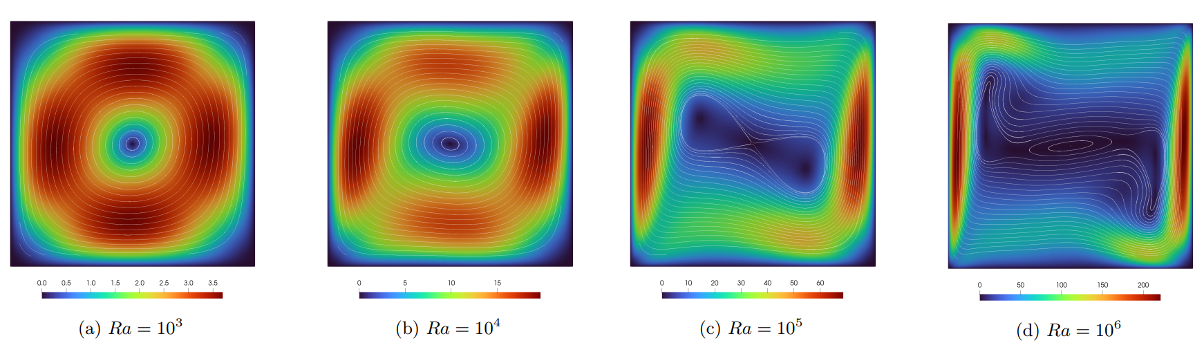
Figure 1: Velocity Field

Figure 2: Temperature

Table 2: Comparison of Cardinal results with the benchmark

Ra	$var element = document.getElementById("moose-equation-896912ca-bf1e-498f-896b-9ba672da8f97");katex.render("10^3", element, {displayMode:false,throwOnError:false});$			$var element = document.getElementById("moose-equation-8541876f-46ce-43f2-93c7-34eb3d1e53f4");katex.render("10^4", element, {displayMode:false,throwOnError:false});$			$var element = document.getElementById("moose-equation-5d51f1c3-c203-4b35-8941-086a323bf6d6");katex.render("10^5", element, {displayMode:false,throwOnError:false});$			$var element = document.getElementById("moose-equation-332a6414-dc60-4896-8640-22fc38bb2de9");katex.render("10^6", element, {displayMode:false,throwOnError:false});$
-	Cardinal	Benchmark	Relative Error	Cardinal	Benchmark	Relative Error	Cardinal	Benchmark	Relative Error	Cardinal	Benchmark	Relative Error
$var element = document.getElementById("moose-equation-0e65547a-b090-413c-8f9b-ded247ed1b56");katex.render("u_{max}", element, {displayMode:false,throwOnError:false});$	3.649	3.649	0.0E+00	16.171	16.178	4.3E-04	34.66	34.73	2.0E-03	64.80	64.63	2.6E-03
$var element = document.getElementById("moose-equation-e4be2fcb-124e-46da-b369-e9a796a8c18a");katex.render("w_{max}", element, {displayMode:false,throwOnError:false});$	3.697	3.697	0.0E+00	19.627	19.617	5.1E-04	68.63	68.59	5.8E-04	220.56	219.36	5.4E-03
$var element = document.getElementById("moose-equation-39fa93fd-fc63-4112-8a36-5a83c40d5d3f");katex.render("\\overline{Nu}", element, {displayMode:false,throwOnError:false});$	1.118	1.118	0.0E+00	2.244	2.243	4.5E-04	4.522	4.519	6.6E-04	8.825	8.800	2.8E-03

A mesh sensitivity study was conducted to ensure that the mesh resolution was sufficient. Table 3 presents the average Nusselt number computed using three different mesh sizes. Since the results obtained with the medium and fine meshes are identical, the medium mesh was selected for the test case. All results reported in Table 2 were computed using this mesh. The medium mesh is shown in Figure 3.

Table 3: Mesh sensitivity

Mesh	Number of Elements	$var element = document.getElementById("moose-equation-7b555df1-7c22-4e0b-ac41-ef606423a7c4");katex.render("\\overline{Nu}", element, {displayMode:false,throwOnError:false});$
Coarse	$var element = document.getElementById("moose-equation-9d0848ab-34da-41bf-a531-4d20c2ff8587");katex.render("377", element, {displayMode:false,throwOnError:false});$	1.121
Medium	$var element = document.getElementById("moose-equation-1bbd1893-d6d1-4e62-846a-daacaf70f8b9");katex.render("377 \\times 4", element, {displayMode:false,throwOnError:false});$	1.118
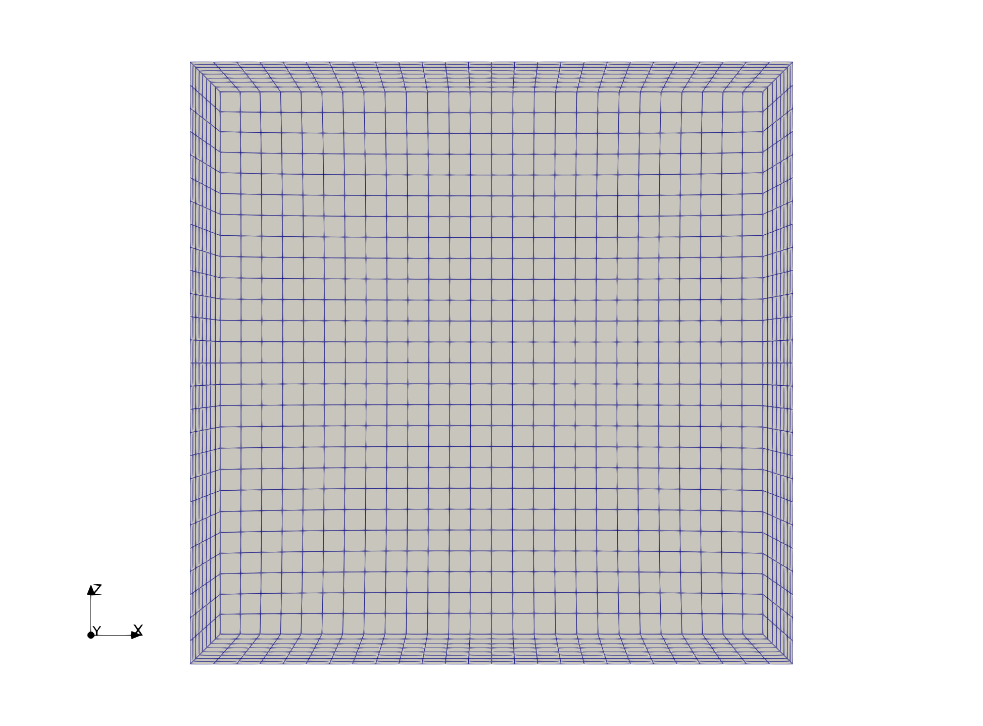
Fine	$var element = document.getElementById("moose-equation-e1e5fe87-c8b1-4f9f-b3b0-246c029bef4b");katex.render("377 \\times 16", element, {displayMode:false,throwOnError:false});$	1.118

Figure 3: Computational mesh (1508 Elements).

Computational Domain
Results