Moving Cylinder (Low-Mach)

The mv_cyl case verifies the low-Mach and moving-mesh capabilities in NekRS using a moving piston in a quasi-two-dimensional domain. The piston is located at $var element = document.getElementById("moose-equation-792ef0e3-d390-4e3a-a774-a3071670fda7");katex.render("y=-L_y", element, {displayMode:false,throwOnError:false});$ , while a stationary wall is located at $var element = document.getElementById("moose-equation-9c5a814d-8397-43ba-8aec-5b155e3b0756");katex.render("y=0", element, {displayMode:false,throwOnError:false});$ . The domain has width $var element = document.getElementById("moose-equation-ad1ce958-38d0-47b3-9c6c-0caee32e3dea");katex.render("L_x", element, {displayMode:false,throwOnError:false});$ , and symmetry boundary conditions are imposed at $var element = document.getElementById("moose-equation-f612c003-bab0-43a1-a0ed-b2a07bc1bbe2");katex.render("x=\\{0,L_x\\}", element, {displayMode:false,throwOnError:false});$ .

Governing equations

Under the ideal-gas assumption, the nondimensional low-Mach governing equations are

(1)var element = document.getElementById("moose-equation-8b937ccf-a283-4ede-a76c-457e802ad7ed");katex.render("\\begin{aligned} \\nabla\\cdot\\vec{v} &= \\frac{1}{T}\\frac{DT}{Dt}-\\frac{1}{p_t}\\frac{dp_t}{dt}=Q, \\\\ \\rho\\left(\\frac{\\partial\\vec{v}}{\\partial t}+\\vec{v}\\cdot\\nabla\\vec{v}\\right) &= -\\nabla p_1+\\frac{1}{Re}\\nabla\\cdot\\left(2\\boldsymbol{\\underline{S}}-\\frac{2}{3}Q\\boldsymbol{\\underline{I}}\\right), \\\\ \\rho c_p\\frac{DT}{Dt} &= \\frac{1}{Pe}\\nabla\\cdot\\nabla T+\\frac{\\gamma-1}{\\gamma}\\frac{dp_t}{dt}, \\\\ p_t &= \\rho T. \\end{aligned}", element, {displayMode:true,throwOnError:false});

Here, $var element = document.getElementById("moose-equation-8c06a170-46bc-456a-a614-56a43c61c01f");katex.render("Q", element, {displayMode:false,throwOnError:false});$ is the thermal divergence, $var element = document.getElementById("moose-equation-a67c20d1-50e2-4acf-986f-2116b547ace8");katex.render("p_t", element, {displayMode:false,throwOnError:false});$ is the thermodynamic pressure, $var element = document.getElementById("moose-equation-7b3f1170-62ef-4935-8369-5e5351687c8e");katex.render("p_1", element, {displayMode:false,throwOnError:false});$ is the hydrodynamic pressure, $var element = document.getElementById("moose-equation-5e7dd376-8782-40b7-9972-f45d8f40c54f");katex.render("\\gamma", element, {displayMode:false,throwOnError:false});$ is the ratio of specific heats, $var element = document.getElementById("moose-equation-32ce8bec-e6cc-42c1-b517-88660b433ea7");katex.render("\\boldsymbol{\\underline{S}}=\\frac{1}{2}\\left(\\nabla\\vec{v}+\\nabla\\vec{v}^{\\,T}\\right)", element, {displayMode:false,throwOnError:false});$ is the strain-rate tensor, and $var element = document.getElementById("moose-equation-1adcfe6e-7ca9-4ecd-a7be-4f343dfe059c");katex.render("\\boldsymbol{\\underline{I}}", element, {displayMode:false,throwOnError:false});$ is the identity tensor. The Reynolds and Péclet numbers are denoted by $var element = document.getElementById("moose-equation-c18dfd1c-96a4-4359-a42e-612664e4b197");katex.render("Re", element, {displayMode:false,throwOnError:false});$ and $var element = document.getElementById("moose-equation-2f3dfdcd-0d9e-4001-8ae2-4d83d2fbf243");katex.render("Pe", element, {displayMode:false,throwOnError:false});$ , respectively.

Analytical solution

The piston is prescribed a sinusoidal velocity,

(2)var element = document.getElementById("moose-equation-f89e2f1f-98e7-4cfb-997e-4d819b458110");katex.render("v_p(t)=A\\sin(\\omega t),", element, {displayMode:true,throwOnError:false});

where $var element = document.getElementById("moose-equation-db4352de-1316-4854-aae2-f3a2900441ed");katex.render("A", element, {displayMode:false,throwOnError:false});$ is the piston velocity amplitude. The flow remains isentropic, and the analytical solution is

(3)var element = document.getElementById("moose-equation-da70e089-29e7-45e1-a9f7-b0f8537465db");katex.render("\\begin{aligned} V(t) &= V_0+A_pA\\frac{\\cos(\\omega t)-1}{\\omega}, \\\\ p_t(t) &= p_0\\left(\\frac{V_0}{V(t)}\\right)^\\gamma, \\\\ \\frac{dp_t}{dt} &= \\gamma p_0A_p\\frac{V_0}{V(t)^{\\gamma+1}}v_p(t), \\\\ y_p(t) &= -\\frac{1}{2}\\left[1+\\cos(\\omega t)\\right], \\\\ Q &= \\left(\\frac{\\gamma-1}{\\gamma}-1\\right)\\frac{1}{p_t(t)}\\frac{dp_t}{dt}, \\\\ \\overline{T}(t) &= p_t(t)^{\\frac{\\gamma-1}{\\gamma}}. \\end{aligned}", element, {displayMode:true,throwOnError:false});

Here, $var element = document.getElementById("moose-equation-6a1eee49-c3b7-41e4-940b-ffed8ebe85fc");katex.render("y_p(t)", element, {displayMode:false,throwOnError:false});$ is the piston location, $var element = document.getElementById("moose-equation-38a8edf2-bc4d-4789-ae26-5bd9ee328fab");katex.render("V_0", element, {displayMode:false,throwOnError:false});$ is the initial domain volume, $var element = document.getElementById("moose-equation-50bcca69-c946-46d2-a54a-731e4d2d025b");katex.render("V(t)", element, {displayMode:false,throwOnError:false});$ is the instantaneous domain volume, $var element = document.getElementById("moose-equation-314dfd17-1843-4e41-b2f3-9e42d70f1085");katex.render("p_0", element, {displayMode:false,throwOnError:false});$ is the initial thermodynamic pressure, $var element = document.getElementById("moose-equation-76f9c1a8-6bc0-40b6-b301-f6d20b1644b3");katex.render("A_p", element, {displayMode:false,throwOnError:false});$ is the piston surface area, and $var element = document.getElementById("moose-equation-09371181-b34b-4a08-b0ce-baf0f6443df3");katex.render("\\overline{T}(t)", element, {displayMode:false,throwOnError:false});$ is the spatially averaged temperature.

Verification criterion

The tests are qualified by evaluating the absolute errors in $var element = document.getElementById("moose-equation-53a1e57f-29ef-4e79-a095-cea99d92e378");katex.render("\\{V(t),dV(t)/dt,p_t(t),dp_t/dt,y_p(t),\\overline{T}(t)\\}", element, {displayMode:false,throwOnError:false});$ at a specified time. The volume, piston-position, and mean-temperature errors are compared with stored reference errors using a normalized regression limit of $var element = document.getElementById("moose-equation-3932f9be-6fee-4c78-b826-1ff0bd70ef6f");katex.render("\\mathrm{CI\\_EPS}=5\\%", element, {displayMode:false,throwOnError:false});$ . Solver modes 3, 5, and 6 additionally require the Cardinal mesh-velocity error to be below $var element = document.getElementById("moose-equation-fa04d512-34f9-47f3-8f94-b1bdd6edada9");katex.render("10^{-11}", element, {displayMode:false,throwOnError:false});$ . Solver modes 1 and 2 use the three physical regression checks in the overall pass criterion, while solver modes 3, 5, and 6 include the mesh-velocity check as well.

For the various tests, the mesh velocity is either prescribed analytically as,

(4)var element = document.getElementById("moose-equation-d014c2be-1ad6-40f6-a3c3-40cabae3b397");katex.render("v_m(y,t)=v_p(t)\\frac{y-y_{\\max}(t)}{y_{\\min}(t)-y_{\\max}(t)}.", element, {displayMode:true,throwOnError:false});

or the mesh motion is computed using the elasticity solver with the piston velocity prescribed as a Dirichlet boundary condition. All routine regression configurations use polynomial order $var element = document.getElementById("moose-equation-5af5a01a-4c62-4266-a942-1a9cf4b33238");katex.render("N=7", element, {displayMode:false,throwOnError:false});$ . The figures below present separate time-step-refinement studies and are not generated by the routine regression tests, which evaluate the qualifying errors at designated time-step sizes. They showcase temporal convergence at this fixed spatial discretization. The tests are organized into various solver modes, as follows:

Mode 1

This solver mode tests:

Low-Mach solver.
Passive scalar solver.
Prescribed moving mesh.

The regression errors are computed at $var element = document.getElementById("moose-equation-190f9318-4941-47fe-8b3e-db7b79fde5d4");katex.render("t=0.1", element, {displayMode:false,throwOnError:false});$ . Figure 1 shows the corresponding time-step-refinement study.

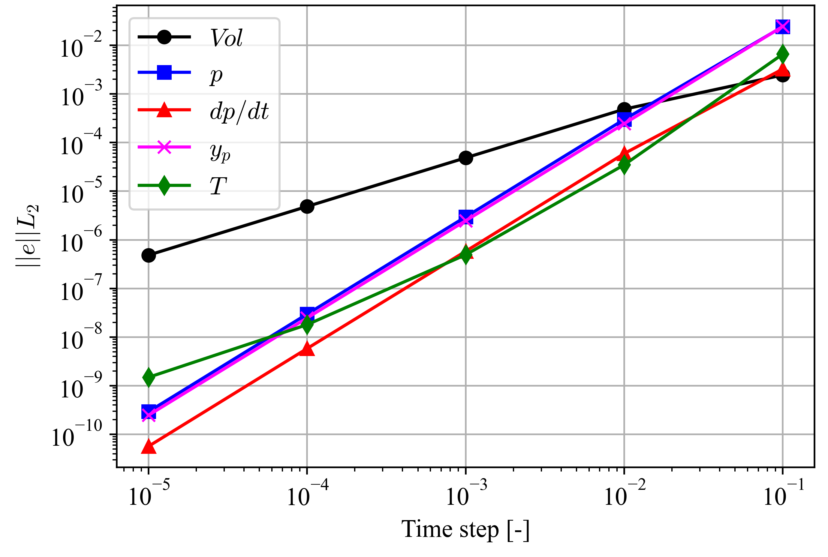
Temporal convergence results for the moving-cylinder case using solver mode 1

Figure 1: Temporal convergence under time-step refinement for solver mode 1; the routine regression test uses polynomial order seven.

Mode 2

This solver mode tests:

All capabilities exercised in solver mode 1.
Characteristic subcycling.

The regression errors are computed at $var element = document.getElementById("moose-equation-d73f1af6-a121-46b7-9011-ee649bcf7cfc");katex.render("t=0.1", element, {displayMode:false,throwOnError:false});$ . Figure 2 shows the corresponding time-step-refinement study.

Temporal convergence results for the moving-cylinder case using solver mode 2

Figure 2: Temporal convergence under time-step refinement for solver mode 2; the routine regression test uses polynomial order seven.

Mode 3

This solver mode tests:

All capabilities exercised in solver mode 2.
Elasticity mesh solver.
Mesh projection.

The regression errors are computed at $var element = document.getElementById("moose-equation-faa61f0c-c1e2-4ee0-8154-d08ef77e5ace");katex.render("t=0.1", element, {displayMode:false,throwOnError:false});$ . Figure 3 shows the corresponding time-step-refinement study.

Temporal convergence results for the moving-cylinder case using solver mode 3

Figure 3: Temporal convergence under time-step refinement for solver mode 3; the routine regression test uses polynomial order seven.

Mode 5

This solver mode verifies the capabilities of solver mode 1 on an unaligned mesh. The regression errors are computed at $var element = document.getElementById("moose-equation-6748c784-d2a2-4385-81c7-bd0bbc08a9af");katex.render("t=0.1", element, {displayMode:false,throwOnError:false});$ . Figure 4 shows the corresponding time-step-refinement study.

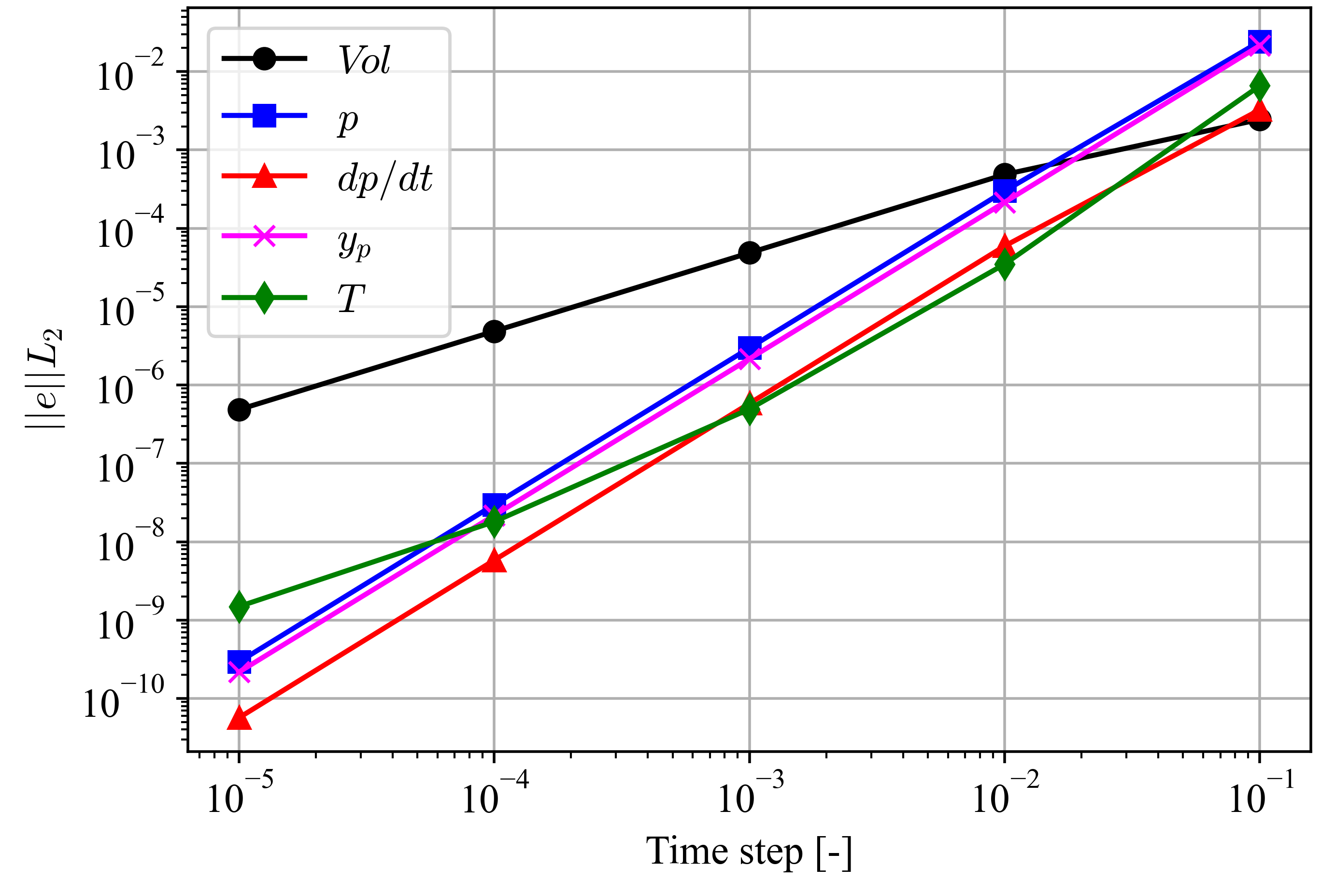
Figure 4: Temporal convergence under time-step refinement for solver mode 5; the routine regression test uses polynomial order seven.

Mode 6

This solver mode verifies the capabilities of solver mode 3 on an unaligned mesh. The regression errors are computed at $var element = document.getElementById("moose-equation-793c8a2b-2477-41c5-9e42-7d2171acdae3");katex.render("t=0.1", element, {displayMode:false,throwOnError:false});$ . Figure 5 shows the corresponding time-step-refinement study.

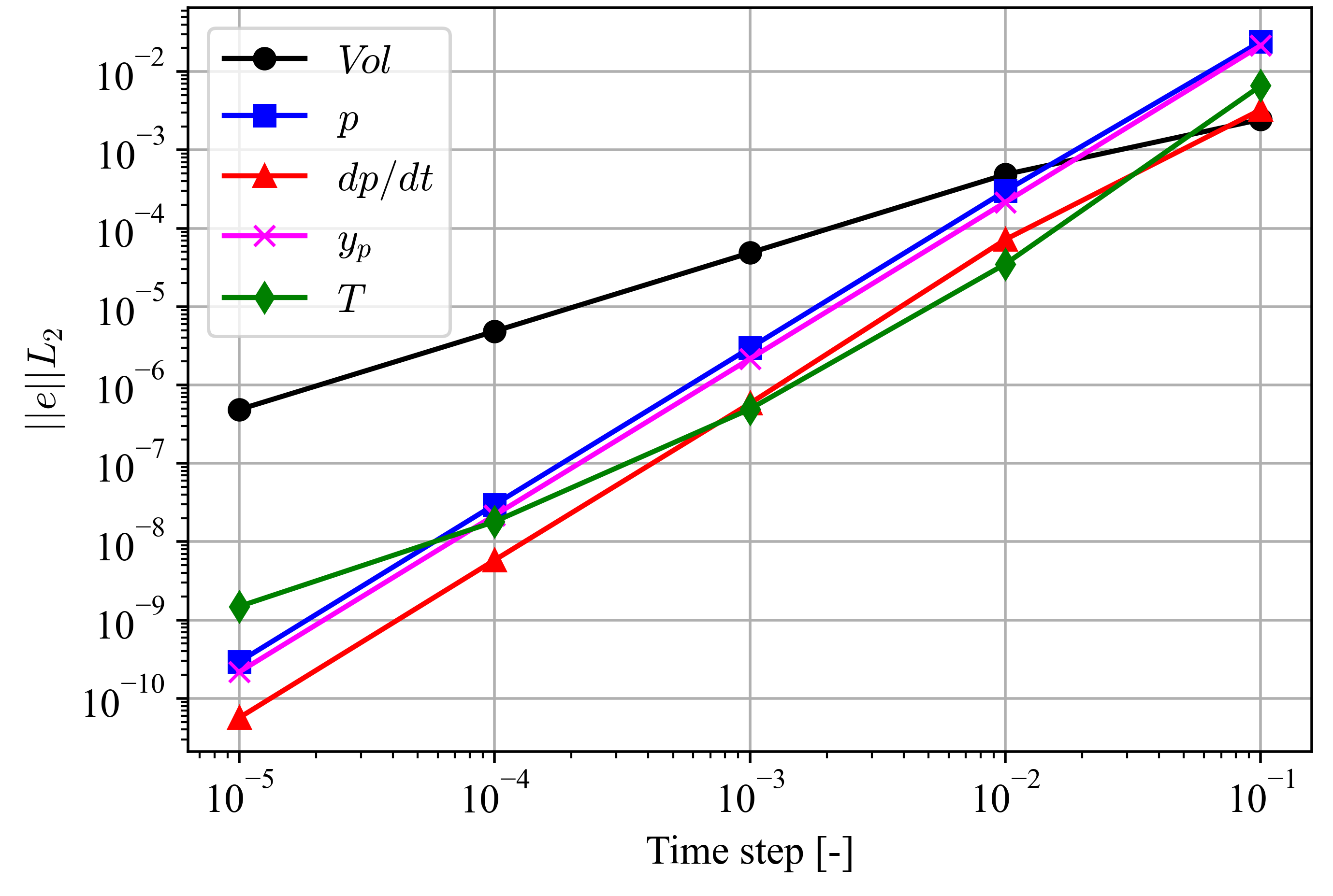
Figure 5: Temporal convergence under time-step refinement for solver mode 6; the routine regression test uses polynomial order seven.

Governing equations
Analytical solution
Verification criterion
Mode 1
Mode 2
Mode 3
Mode 5
Mode 6