Low-Mach Compressible Flow
The low-Mach governing equations are obtained by filtering acoustic waves from the fully compressible Navier–Stokes equations. The pressure is decomposed into a spatially uniform, leading-order thermodynamic component and a first-order hydrodynamic component that appears in the momentum equation (Tomboulides et al., 1997). The low-Mach formulation is applicable to low-speed flows with significant density variations, such as reactive flows and natural convection, where thermal expansion must be captured while acoustic waves are neglected.
Problem description
The lowMach case is adopted from Tomboulides et al. (Tomboulides and Orzag, 1998). The problem is a nontrivial, quasi-two-dimensional verification problem derived from the following one-dimensional system:
(1)Here, is the temperature, is the -component of velocity, is the thermal diffusivity, is the Reynolds number, is the Prandtl number, is the volumetric heat source, is the kinematic viscosity, is the hydrodynamic pressure, is the density, and is the spatial coordinate.
Computational domain
The problem is solved on the domain and . Periodic boundary conditions are applied in the and directions.
Analytical solution
The volumetric heat source introduced by Tomboulides et al. (Tomboulides and Orzag, 1998) is
(2)The exact solution of the system is the smooth step profile
(3)where is a user-specified parameter that controls the sharpness of the solution profile. Dirichlet boundary conditions are imposed at and using the analytical solution.
Verification criteria and results
Two simulations are performed using a polynomial order of seven; the second simulation enables characteristic subcycling for the fluid and temperature solvers. Errors are evaluated at . The test evaluates errors in velocity, temperature, and hydrodynamic pressure. For the solver mode without characteristic subcycling, the stored reference values are , , and , respectively. For the solver mode with characteristic subcycling, the corresponding reference values are , , and . Each normalized difference between a computed error and its stored reference value must be below . Figure 1 and Figure 2 present separate -refinement studies for the solver modes without and with characteristic subcycling. These refinement sweeps are not part of the routine regression tests, which use polynomial order ; the figures showcase spectral convergence of the velocity, hydrodynamic pressure, and temperature fields and provide additional evidence of the low-Mach solver's accuracy.
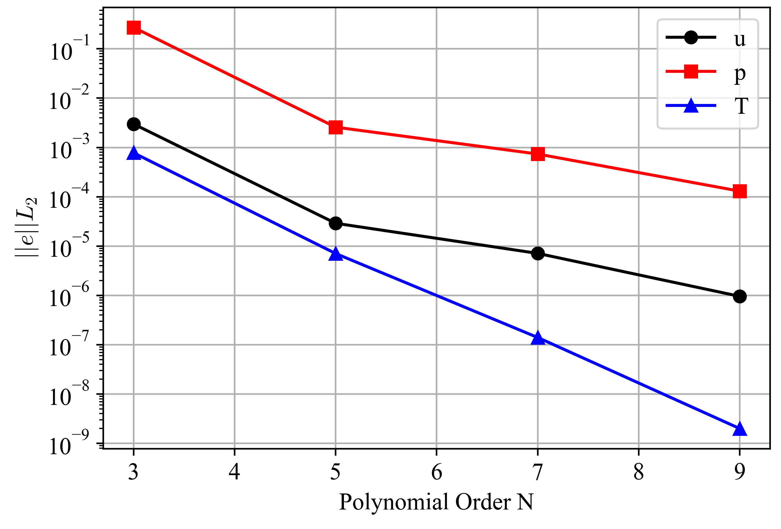
Figure 1: Spectral convergence under p refinement without characteristic subcycling; the routine regression test uses polynomial order seven.
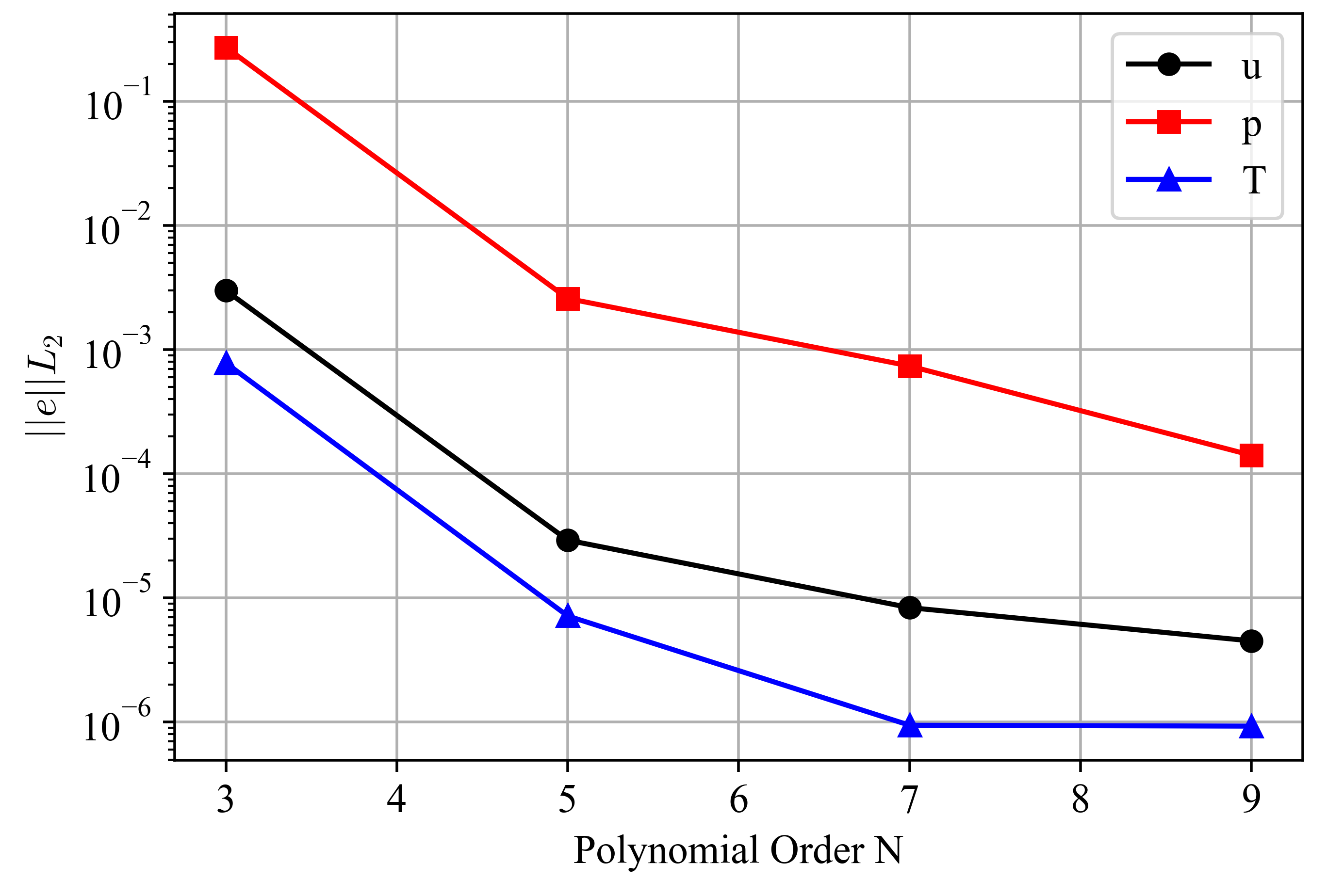
Figure 2: Spectral convergence under p refinement with characteristic subcycling; the routine regression test uses polynomial order seven.
References
- AG Tomboulides, JCY Lee, and Steven A Orszag.
Numerical simulation of low mach number reactive flows.
Journal of Scientific Computing, 12(2):139–167, 1997.[Export]
- Ananias G Tomboulides and Steven A Orzag.
A quasi-two-dimensional benchmark problem for low mach number compressible codes.
Journal of Computational Physics, 146(2):691–706, 1998.[Export]