Ethier Flow

This case is adopted from the nontrivial exact solution of the three-dimensional incompressible Navier–Stokes equations developed by Ethier and Steinman (Ethier and Steinman, 1994) for benchmarking incompressible CFD solvers. The Ethier solution is also used to verify the passive scalar solvers in NekRS. This is accomplished by selecting the $var element = document.getElementById("moose-equation-2f76d17a-f782-4c25-9a0f-e5a2bf99c2f1");katex.render("x", element, {displayMode:false,throwOnError:false});$ -component of the velocity field as the transported passive scalar and using the pressure term from the momentum equation as its source term, making the passive scalar transport equation identical to the $var element = document.getElementById("moose-equation-5958297c-5095-47fb-aeb2-2cafd4e01686");katex.render("x", element, {displayMode:false,throwOnError:false});$ -momentum equation. Because the analytical solution is known throughout the domain and for all times, both the incompressible flow and passive scalar solvers can be verified using only a few time steps, minimizing the computational cost of the tests. Consequently, the ethier case verifies several NekRS capabilities through multiple different tests and solver modes.

Computational domain

The problem is solved in the cubic domain

(1)var element = document.getElementById("moose-equation-499dc85f-0e00-4427-afde-49057376c94b");katex.render("(x,y,z)\\in[-1,1]^3.", element, {displayMode:true,throwOnError:false});

Dirichlet boundary conditions obtained from the analytical solution are imposed for the velocity field. Dirichlet and Neumann boundary conditions are imposed for the passive scalars $var element = document.getElementById("moose-equation-0241a561-d639-43d8-9392-fdb405bcf6a7");katex.render("s_1", element, {displayMode:false,throwOnError:false});$ and $var element = document.getElementById("moose-equation-bccf773a-e587-43a6-8286-a97a4e6014ae");katex.render("s_2", element, {displayMode:false,throwOnError:false});$ , respectively.

Analytical solution

The analytical velocity and pressure fields of Ethier and Steinman (Ethier and Steinman, 1994) are

(2)var element = document.getElementById("moose-equation-f03b0f0b-7c83-4f7e-abd7-cb7e1249026f");katex.render("\\begin{aligned} u &= -a\\left[ e^{ax}\\sin(ay+dz) +e^{az}\\cos(ax+dy) \\right]e^{-d^2t}, \\\\ v &= -a\\left[ e^{ay}\\sin(az+dx) +e^{ax}\\cos(ay+dz) \\right]e^{-d^2t}, \\\\ w &= -a\\left[ e^{az}\\sin(ax+dy) +e^{ay}\\cos(az+dx) \\right]e^{-d^2t}, \\\\ p &= -\\frac{a^2}{2} \\left[ e^{2ax}+e^{2ay}+e^{2az} +2\\sin(ax+dy)\\cos(az+dx)e^{a(y+z)} \\right. \\\\ &\\qquad\\left. +2\\sin(ay+dz)\\cos(ax+dy)e^{a(z+x)} +2\\sin(az+dx)\\cos(ay+dz)e^{a(x+y)} \\right]e^{-2d^2t}, \\end{aligned}", element, {displayMode:true,throwOnError:false});

where $var element = document.getElementById("moose-equation-513b21b8-72f2-4d7e-ae39-b9326c0f61ea");katex.render("a", element, {displayMode:false,throwOnError:false});$ and $var element = document.getElementById("moose-equation-799bf242-30a7-4027-995d-a3c2aed05010");katex.render("d", element, {displayMode:false,throwOnError:false});$ are user-specified parameters, $var element = document.getElementById("moose-equation-730aba1b-49d2-48f0-887e-42ef7b74fca1");katex.render("\\{x,y,z\\}", element, {displayMode:false,throwOnError:false});$ are the spatial coordinates, $var element = document.getElementById("moose-equation-ead10197-821a-4fe1-9bc5-0c98016726e6");katex.render("\\{u,v,w\\}", element, {displayMode:false,throwOnError:false});$ are the velocity components, $var element = document.getElementById("moose-equation-554d56dd-4469-4847-b23f-9fe558c9eda2");katex.render("p", element, {displayMode:false,throwOnError:false});$ is the pressure, and $var element = document.getElementById("moose-equation-b8a7f42a-0b68-47f1-a28a-2aa544226193");katex.render("t", element, {displayMode:false,throwOnError:false});$ is time. For the passive scalar verification tests, the transported analytical variable is the $var element = document.getElementById("moose-equation-0be7838c-01bf-442a-bc55-bfb0f61ad93f");katex.render("x", element, {displayMode:false,throwOnError:false});$ -component of velocity, $var element = document.getElementById("moose-equation-11e6011e-41f2-47c2-98f3-becbe941bb4a");katex.render("u", element, {displayMode:false,throwOnError:false});$ .

Verification criteria

The solution fields evaluated are

(3)var element = document.getElementById("moose-equation-e01f9c6d-34fe-408a-835e-c63511ac89e8");katex.render("\\phi\\in\\{u,p,s_1,s_2\\},", element, {displayMode:true,throwOnError:false});

corresponding to the $var element = document.getElementById("moose-equation-3b6b717b-c9cb-414d-8b96-fe1799a409a8");katex.render("x", element, {displayMode:false,throwOnError:false});$ -velocity, pressure, and two passive scalar fields. For each evaluated field, the volume-integrated error norm is

(4)var element = document.getElementById("moose-equation-6d3e863f-4c79-4ed2-b59d-4fb23d997991");katex.render("\\varepsilon_\\phi = \\left\\lVert\\phi-\\phi_{\\mathrm{exact}}\\right\\rVert_{L_2(\\Omega)} = \\left[ \\int_\\Omega \\left(\\phi-\\phi_{\\mathrm{exact}}\\right)^2 \\,d\\Omega \\right]^{1/2}.", element, {displayMode:true,throwOnError:false});

The routine regression tests use polynomial order $var element = document.getElementById("moose-equation-49352abd-8c8c-4ebf-ae9e-32b0b2250783");katex.render("N=9", element, {displayMode:false,throwOnError:false});$ for every qualifying solver mode. The figures below are generated from separate $var element = document.getElementById("moose-equation-1a043e1f-1545-48d0-8b0c-b9e78d4cd9c8");katex.render("p", element, {displayMode:false,throwOnError:false});$ -refinement studies and are not part of the routine regression tests; they demonstrate spectral convergence as the polynomial order increases and provide additional evidence of the accuracy and consistency of the flow and passive scalar solvers. The tests also monitor the numbers of iterations required for convergence of the velocity, pressure, and passive scalar solvers. The specific NekRS capabilities verified by each test are described below. The tests are organized into different solver modes as follows:

The qualifying postprocessor is evaluated at the final time and requires every enabled error norm to be below its mode-specific tolerance, or below $var element = document.getElementById("moose-equation-b9258567-1866-4f30-875c-fabbe9719960");katex.render("10^{-11}", element, {displayMode:false,throwOnError:false});$ when that fallback criterion is satisfied. The tolerances for the tested solver modes are summarized in Table 1. Solver mode 13 is the scalar-only case, and solver mode 12 intentionally disables the temperature solve.

Table 1: Pass criteria for the tested Ethier solver modes.

Solver mode	Velocity error	Pressure error	Temperature error	Passive-scalar error
2, 3, 11, 14	$var element = document.getElementById("moose-equation-7e65ba2d-265d-4f5a-90cd-dc927f2ad70e");katex.render("4.78\\times10^{-8}", element, {displayMode:false,throwOnError:false});$	$var element = document.getElementById("moose-equation-48af7830-5c83-4342-8b96-bc4601e471ef");katex.render("1.08\\times10^{-7}", element, {displayMode:false,throwOnError:false});$	$var element = document.getElementById("moose-equation-19629c98-8e34-46a2-ad7e-6af939845718");katex.render("9.48\\times10^{-10}", element, {displayMode:false,throwOnError:false});$	$var element = document.getElementById("moose-equation-d7c3572c-5822-416c-992c-3184977e1ced");katex.render("1.07\\times10^{-9}", element, {displayMode:false,throwOnError:false});$
4	$var element = document.getElementById("moose-equation-b242f65b-9f7f-44d3-abe6-ad9f125dd157");katex.render("5.90\\times10^{-8}", element, {displayMode:false,throwOnError:false});$	$var element = document.getElementById("moose-equation-98a6c781-52b1-499b-aa90-9c69d9c2c3d1");katex.render("9.91\\times10^{-8}", element, {displayMode:false,throwOnError:false});$	$var element = document.getElementById("moose-equation-c304bf10-c803-413d-bcc6-7478b91006a4");katex.render("2.09\\times10^{-9}", element, {displayMode:false,throwOnError:false});$	$var element = document.getElementById("moose-equation-0d1a6763-1fbe-4d78-9b77-74cb4df2a893");katex.render("2.63\\times10^{-9}", element, {displayMode:false,throwOnError:false});$
5	$var element = document.getElementById("moose-equation-13f68d8c-4934-4324-b4c1-f88e7ab05ad9");katex.render("2.21\\times10^{-5}", element, {displayMode:false,throwOnError:false});$	$var element = document.getElementById("moose-equation-5cf64b70-81ef-4107-bed3-281dd9d6f823");katex.render("5.89\\times10^{-5}", element, {displayMode:false,throwOnError:false});$	$var element = document.getElementById("moose-equation-fcf3c10a-673f-4662-8c51-4c9102b084da");katex.render("1.04\\times10^{-5}", element, {displayMode:false,throwOnError:false});$	$var element = document.getElementById("moose-equation-5f1b3fd2-4390-4011-8874-a705525aed01");katex.render("1.32\\times10^{-5}", element, {displayMode:false,throwOnError:false});$
6	$var element = document.getElementById("moose-equation-0c11d998-bfb8-4ab4-a095-b0e5017a5cf8");katex.render("1.17\\times10^{-5}", element, {displayMode:false,throwOnError:false});$	$var element = document.getElementById("moose-equation-f54e965e-dccc-4db0-927e-83f5452602c8");katex.render("4.67\\times10^{-5}", element, {displayMode:false,throwOnError:false});$	$var element = document.getElementById("moose-equation-580f6558-c5c6-4d10-833b-cc91a0d797a9");katex.render("5.20\\times10^{-6}", element, {displayMode:false,throwOnError:false});$	$var element = document.getElementById("moose-equation-337c1ab8-d94e-4772-a96b-516c3229e38c");katex.render("6.14\\times10^{-6}", element, {displayMode:false,throwOnError:false});$
7	$var element = document.getElementById("moose-equation-21e2f3d5-998f-48c1-a91c-5fa0612e76c1");katex.render("2.51\\times10^{-8}", element, {displayMode:false,throwOnError:false});$	$var element = document.getElementById("moose-equation-734079c8-f249-4456-a934-11a8060c0c50");katex.render("1.93\\times10^{-6}", element, {displayMode:false,throwOnError:false});$	$var element = document.getElementById("moose-equation-5f1cdf61-d7a2-4829-b0a3-d6d656ff7d90");katex.render("2.90\\times10^{-11}", element, {displayMode:false,throwOnError:false});$	$var element = document.getElementById("moose-equation-7895222e-85da-4da4-af61-77587350db16");katex.render("3.08\\times10^{-11}", element, {displayMode:false,throwOnError:false});$
8	$var element = document.getElementById("moose-equation-f83a6b4a-2aaa-4dd4-a3f9-834e9b763ce2");katex.render("8.68\\times10^{-6}", element, {displayMode:false,throwOnError:false});$	$var element = document.getElementById("moose-equation-1c7f7bf5-ab5f-4274-9f11-4b8e76172e6d");katex.render("9.93\\times10^{-3}", element, {displayMode:false,throwOnError:false});$	$var element = document.getElementById("moose-equation-90567568-b24f-4990-b0df-1c61d1cfef56");katex.render("7.29\\times10^{-6}", element, {displayMode:false,throwOnError:false});$	$var element = document.getElementById("moose-equation-bbf43bf2-caa8-427e-8f60-935d5c27d0be");katex.render("7.96\\times10^{-6}", element, {displayMode:false,throwOnError:false});$
9, 10	$var element = document.getElementById("moose-equation-20f3b186-7280-481e-83ba-1c488d54b535");katex.render("4.79\\times10^{-8}", element, {displayMode:false,throwOnError:false});$	$var element = document.getElementById("moose-equation-6cbb147e-66b4-447e-8400-c2d08df7c2ec");katex.render("1.08\\times10^{-7}", element, {displayMode:false,throwOnError:false});$	$var element = document.getElementById("moose-equation-f0a4a77d-0e59-44e4-b2a4-49e06ce85593");katex.render("8.77\\times10^{-10}", element, {displayMode:false,throwOnError:false});$	$var element = document.getElementById("moose-equation-1d13ad30-963d-417d-92ac-c098f8e5af23");katex.render("1.02\\times10^{-9}", element, {displayMode:false,throwOnError:false});$
12	$var element = document.getElementById("moose-equation-a8792649-aa78-4403-9a41-d30a3c8d6de4");katex.render("4.78\\times10^{-8}", element, {displayMode:false,throwOnError:false});$	$var element = document.getElementById("moose-equation-17660d8a-4c53-4a5c-8435-58c417e52b99");katex.render("1.08\\times10^{-7}", element, {displayMode:false,throwOnError:false});$	–	$var element = document.getElementById("moose-equation-50895679-8eb0-402c-a822-b43185bf92f0");katex.render("1.07\\times10^{-9}", element, {displayMode:false,throwOnError:false});$
13	–	–	–	$var element = document.getElementById("moose-equation-950acc9a-fa33-4835-865d-ff522ce0d758");katex.render("1.53\\times10^{-5}", element, {displayMode:false,throwOnError:false});$

Mode 2

This solver mode verifies:

Incompressible Navier–Stokes and passive scalar solvers.
Block velocity solver.
Characteristic subcycling.

The regression error is evaluated at $var element = document.getElementById("moose-equation-cd267507-3684-4535-a35f-372988a06a6b");katex.render("t=0.06", element, {displayMode:false,throwOnError:false});$ . Figure 1 shows the corresponding $var element = document.getElementById("moose-equation-0dd25a9a-a133-4a20-aa52-34e01cfb87f7");katex.render("p", element, {displayMode:false,throwOnError:false});$ -refinement study.

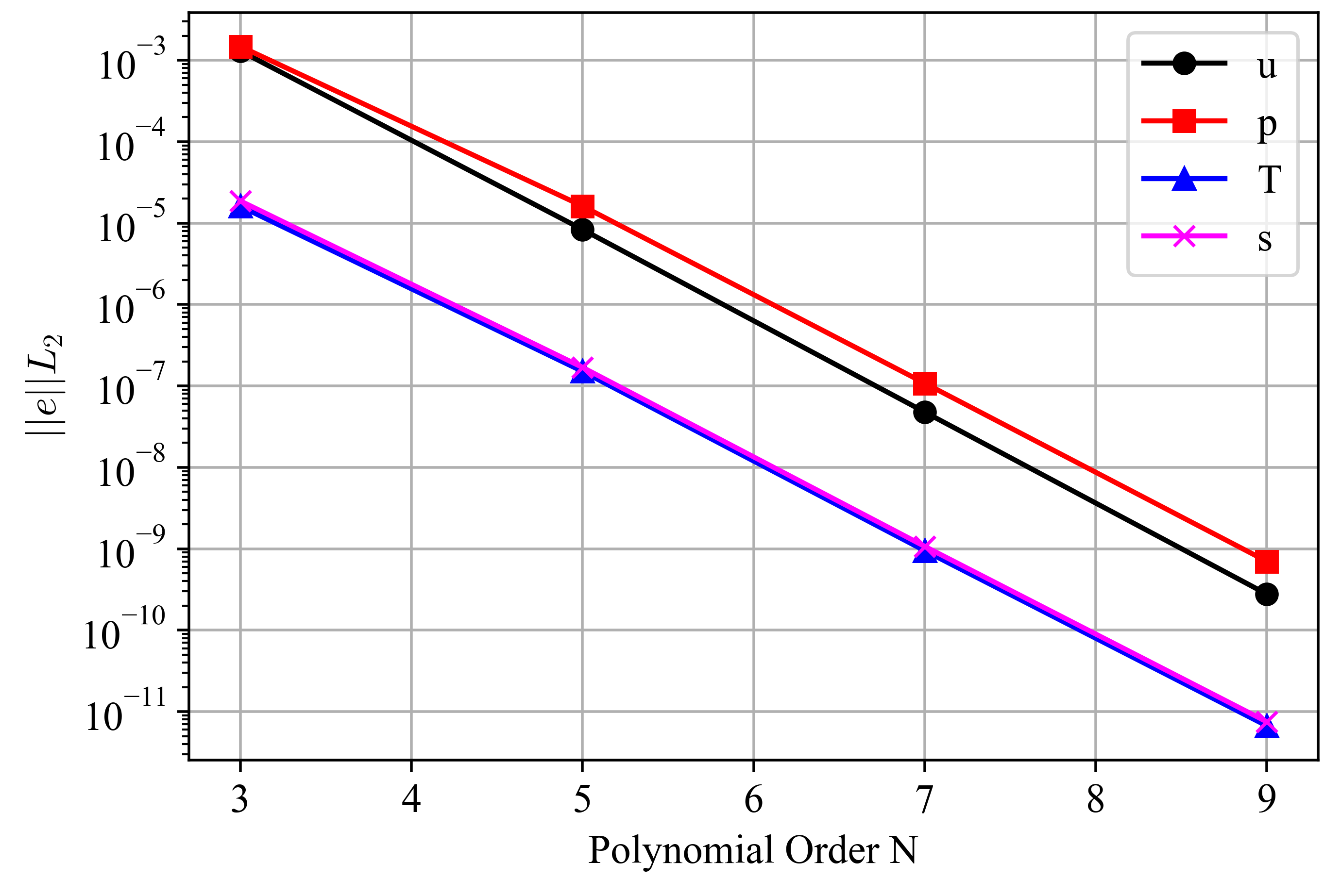
Spectral convergence of the Ethier solution errors using solver mode 2

Figure 1: Spectral convergence under p refinement for the ethier case using solver mode 2; the routine regression test uses polynomial order nine.

Mode 3

This solver mode verifies:

Velocity and pressure projection.
SEMFEM (low-order finite element) pressure preconditioner.

The regression error is evaluated at $var element = document.getElementById("moose-equation-55fa06e3-7bb6-48f9-9661-161e53d62497");katex.render("t=0.06", element, {displayMode:false,throwOnError:false});$ . Figure 2 shows the corresponding $var element = document.getElementById("moose-equation-be0a4609-7ad1-42a5-94ad-a7bbe9fd6ca0");katex.render("p", element, {displayMode:false,throwOnError:false});$ -refinement study.

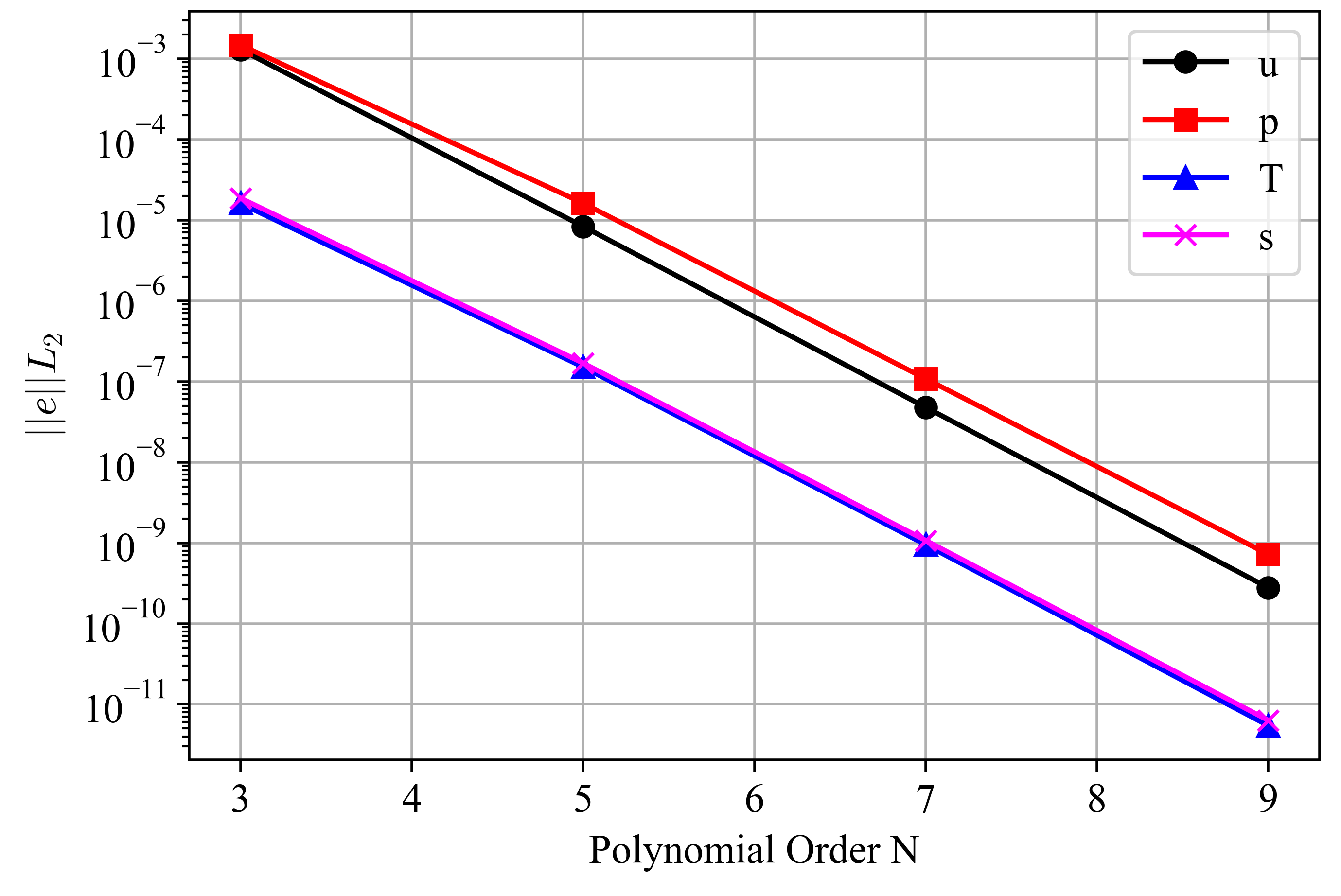
Spectral convergence of the Ethier solution errors using solver mode 3

Figure 2: Spectral convergence under p refinement for the ethier case using solver mode 3; the routine regression test uses polynomial order nine.

Mode 4

This solver mode verifies:

Incompressible Navier–Stokes and passive scalar solvers.
Block velocity solver.
Characteristic subcycling.
Velocity and pressure projection.

The regression error is evaluated at $var element = document.getElementById("moose-equation-5a3aec02-b6b4-4ffe-aa7c-1599dfee2168");katex.render("t=0.2", element, {displayMode:false,throwOnError:false});$ . Figure 3 shows the corresponding $var element = document.getElementById("moose-equation-f6cea81f-b437-4bd9-a963-dcea5cffc019");katex.render("p", element, {displayMode:false,throwOnError:false});$ -refinement study.

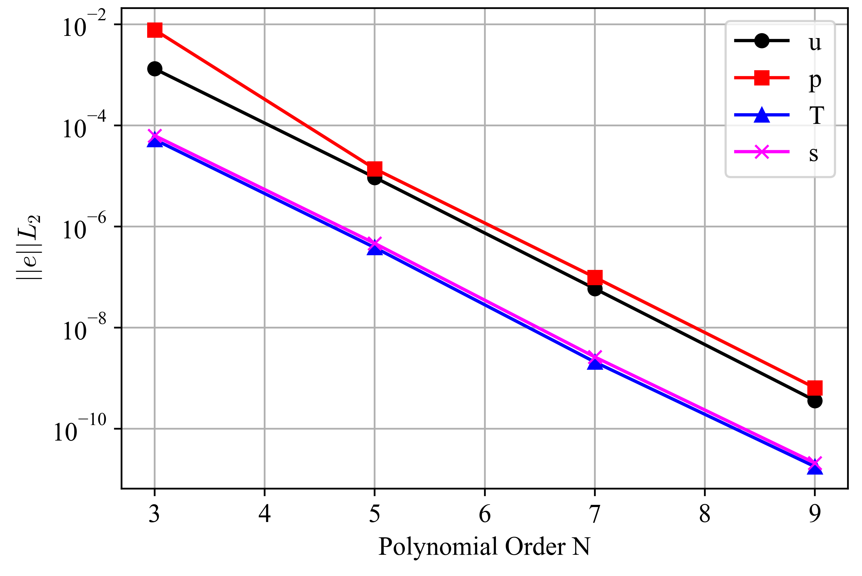
Spectral convergence of the Ethier solution errors using solver mode 4

Figure 3: Spectral convergence under p refinement for the ethier case using solver mode 4; the routine regression test uses polynomial order nine.

Mode 5

This solver mode verifies:

Moving-mesh formulation.
Block velocity solver.

The regression error is evaluated at $var element = document.getElementById("moose-equation-cbc7c9f7-033b-4bd4-afaf-1bc44b791426");katex.render("t=0.2", element, {displayMode:false,throwOnError:false});$ . Figure 4 shows the corresponding $var element = document.getElementById("moose-equation-d390ce8f-2f31-4365-85ea-879945863955");katex.render("p", element, {displayMode:false,throwOnError:false});$ -refinement study.

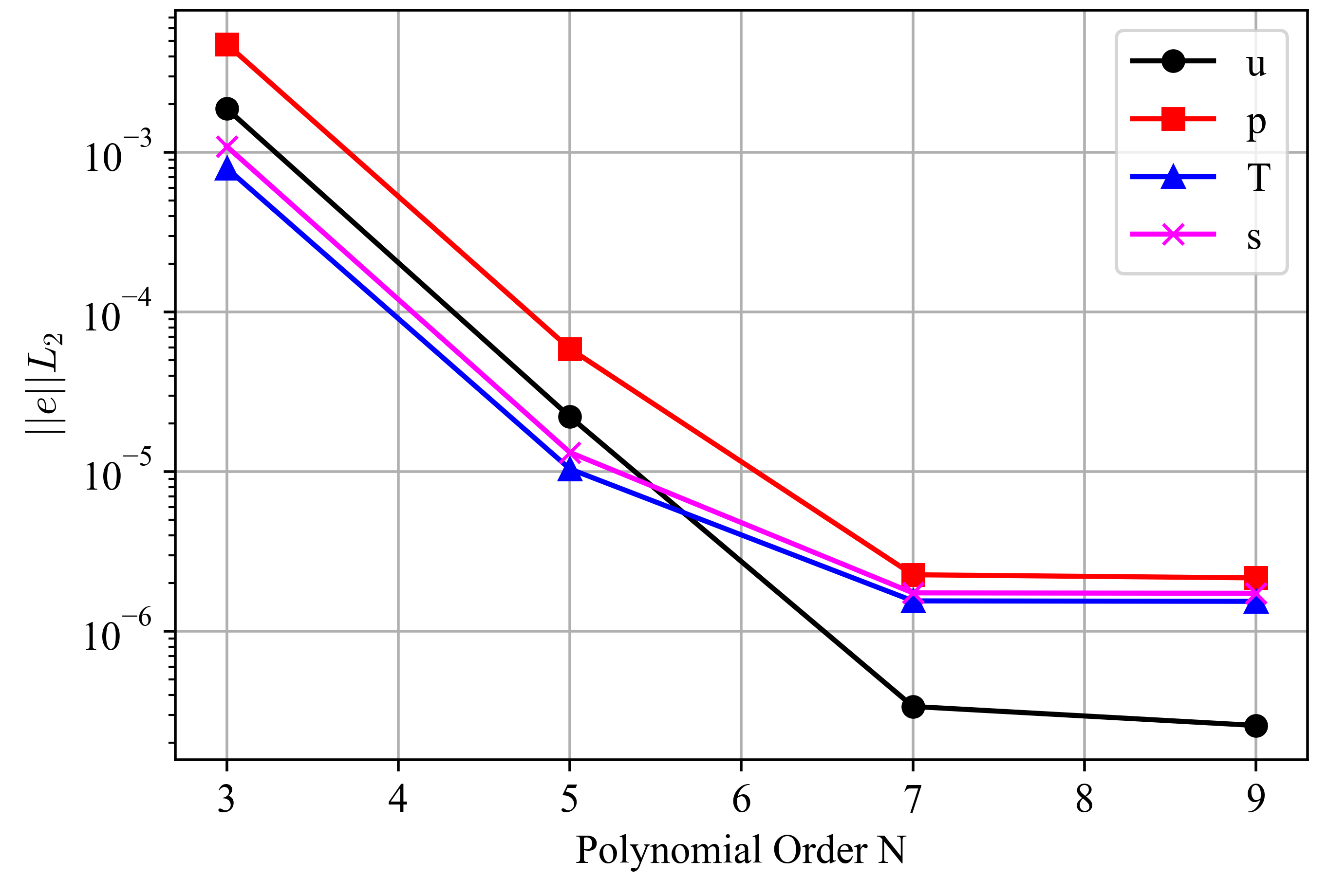
Spectral convergence of the Ethier solution errors using solver mode 5

Figure 4: Spectral convergence under p refinement for the ethier case using solver mode 5; the routine regression test uses polynomial order nine.

Mode 6

This solver mode verifies:

Moving-mesh formulation.
Block velocity solver.
Characteristic subcycling.

The regression error is evaluated at $var element = document.getElementById("moose-equation-a13383b7-eaf6-495c-8236-bc33cea2d045");katex.render("t=0.2", element, {displayMode:false,throwOnError:false});$ . Figure 5 shows the corresponding $var element = document.getElementById("moose-equation-5cf6a1f5-964f-4f2f-a9a8-b24c8e3365a1");katex.render("p", element, {displayMode:false,throwOnError:false});$ -refinement study.

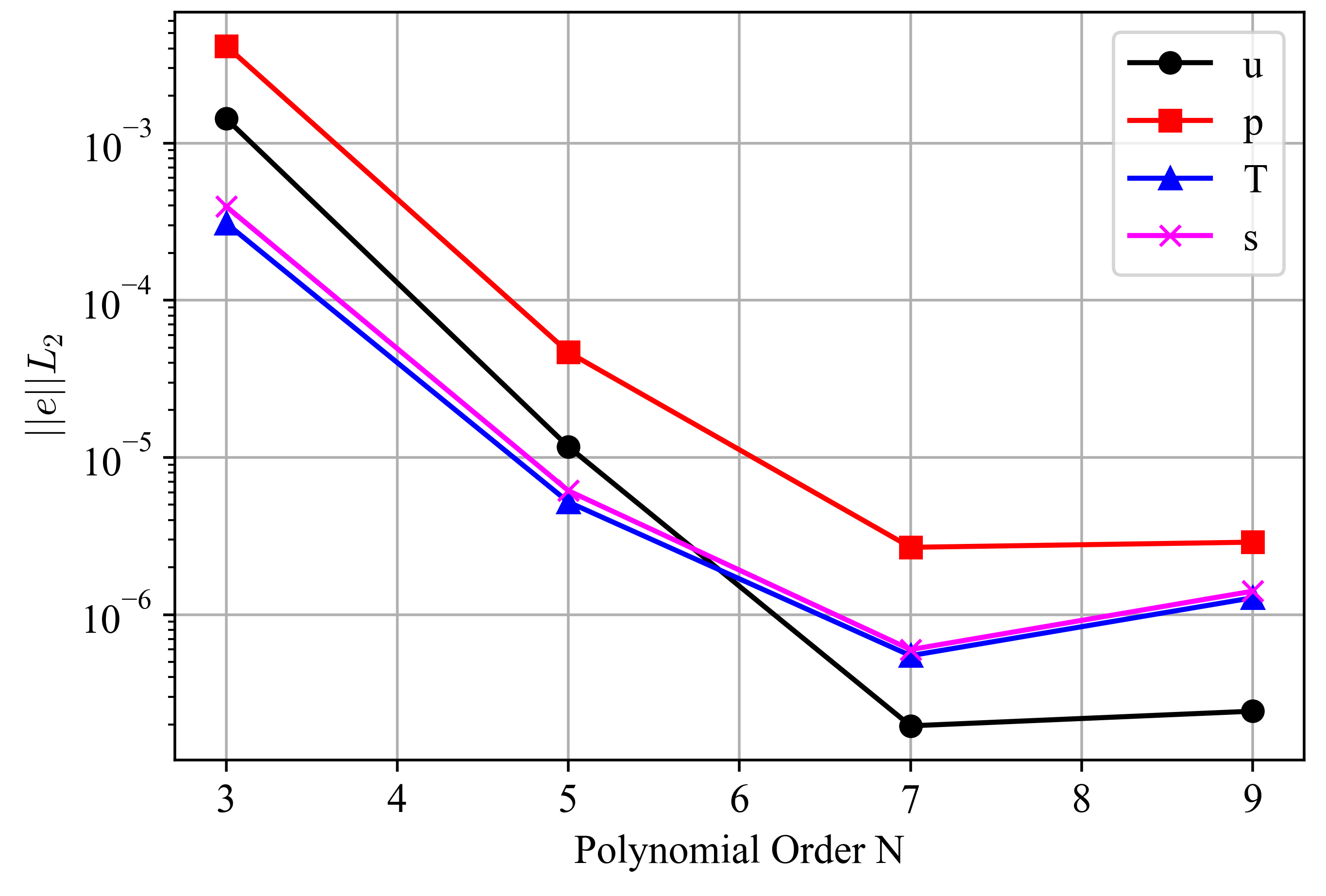
Spectral convergence of the Ethier solution errors using solver mode 6

Figure 5: Spectral convergence under p refinement for the ethier case using solver mode 6; the routine regression test uses polynomial order nine.

Mode 7

This solver mode verifies:

Velocity and pressure projection.
Jacobi pressure preconditioner.

The regression error is evaluated at $var element = document.getElementById("moose-equation-d2c88879-4553-422d-8b07-fa129988de3b");katex.render("t=0.012", element, {displayMode:false,throwOnError:false});$ . Figure 6 shows the corresponding $var element = document.getElementById("moose-equation-ac427bb4-c092-451a-9725-3938b8f103c9");katex.render("p", element, {displayMode:false,throwOnError:false});$ -refinement study.

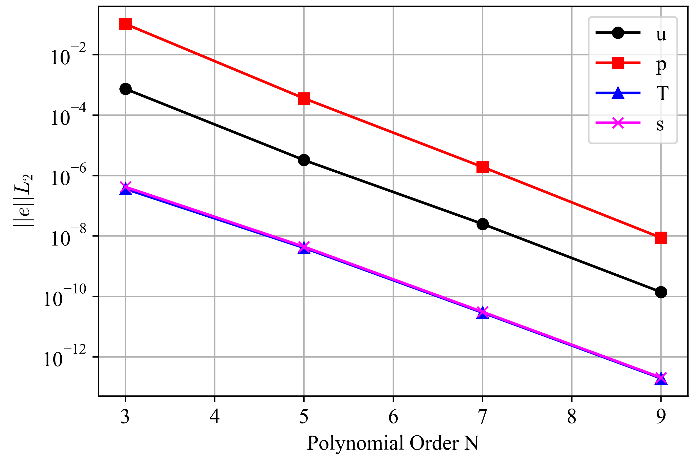
Spectral convergence of the Ethier solution errors using solver mode 7

Figure 6: Spectral convergence under p refinement for the ethier case using solver mode 7; the routine regression test uses polynomial order nine.

Mode 8

This solver mode verifies:

Pressure projection.
Adaptive time stepping.
Compliance of the final CFL number with its specified target.
The expected number of time steps.

The regression error is evaluated at $var element = document.getElementById("moose-equation-28df6b82-bf8b-44b8-b4d4-88563d8e1023");katex.render("t=0.2", element, {displayMode:false,throwOnError:false});$ . Figure 7 shows the corresponding $var element = document.getElementById("moose-equation-48078dbd-6023-4863-8dd2-90b8e66a26db");katex.render("p", element, {displayMode:false,throwOnError:false});$ -refinement study.

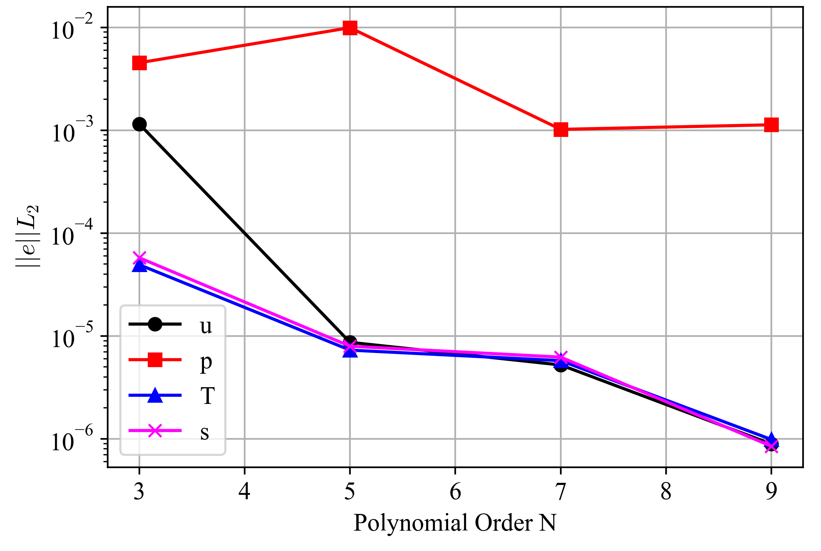
Spectral convergence of the Ethier solution errors using solver mode 8

Figure 7: Spectral convergence under p refinement for the ethier case using solver mode 8; the routine regression test uses polynomial order nine.

Mode 9

This solver mode verifies:

Convective advection formulation without dealiasing.
Block velocity solver.
Characteristic subcycling.
Velocity and pressure projection.

The regression error is evaluated at $var element = document.getElementById("moose-equation-334e3ac2-77d6-41d2-baf7-f00ba3fff0e5");katex.render("t=0.06", element, {displayMode:false,throwOnError:false});$ . Figure 8 shows the corresponding $var element = document.getElementById("moose-equation-13347676-af88-46ff-92f3-a3e163b32eee");katex.render("p", element, {displayMode:false,throwOnError:false});$ -refinement study.

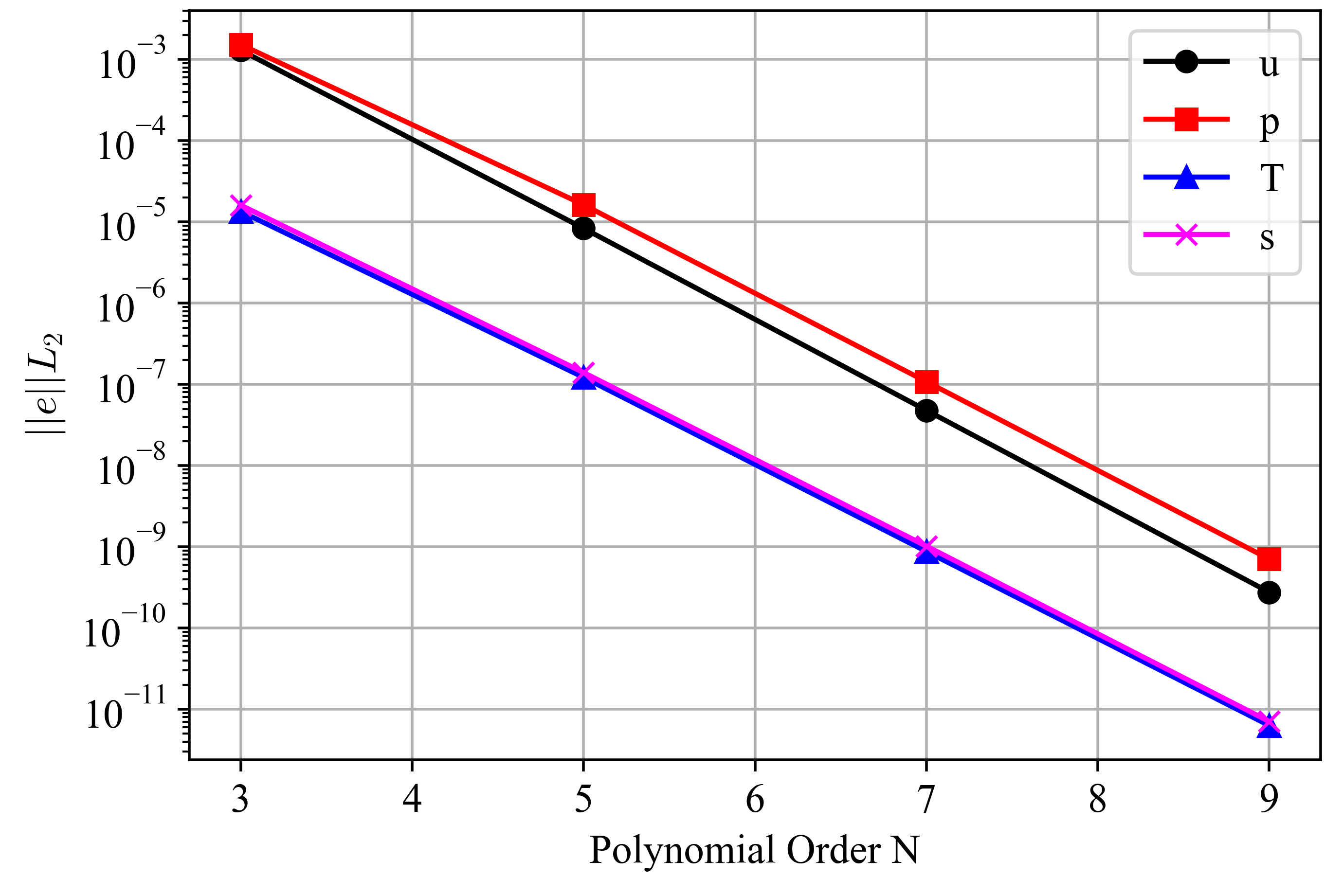
Spectral convergence of the Ethier solution errors using solver mode 9

Figure 8: Spectral convergence under p refinement for the ethier case using solver mode 9; the routine regression test uses polynomial order nine.

Mode 10

This solver mode verifies:

Convective advection formulation without dealiasing.
Block velocity solver.
Velocity and pressure projection.

The regression error is evaluated at $var element = document.getElementById("moose-equation-e41d960b-2776-472e-b63d-85f30947a0e7");katex.render("t=0.06", element, {displayMode:false,throwOnError:false});$ . Figure 9 shows the corresponding $var element = document.getElementById("moose-equation-6bd152ed-0ed5-4b96-9a70-bbb531db77ca");katex.render("p", element, {displayMode:false,throwOnError:false});$ -refinement study.

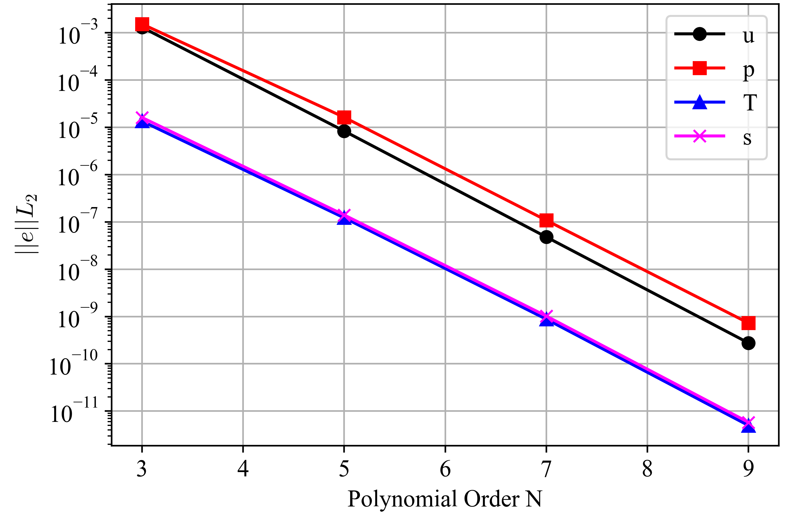
Spectral convergence of the Ethier solution errors using solver mode 10

Figure 9: Spectral convergence under p refinement for the ethier case using solver mode 10; the routine regression test uses polynomial order nine.

Mode 11

This solver mode verifies:

Chebyshev-accelerated damped-Jacobi pressure multigrid smoother.
Block velocity solver.
Characteristic subcycling.
Pressure projection.

The regression error is evaluated at $var element = document.getElementById("moose-equation-d37c0c3d-03b4-4b44-95b4-b34105057866");katex.render("t=0.06", element, {displayMode:false,throwOnError:false});$ . Figure 10 shows the corresponding $var element = document.getElementById("moose-equation-2c917a42-a5a0-474f-8b70-bb423f7323bd");katex.render("p", element, {displayMode:false,throwOnError:false});$ -refinement study.

Spectral convergence of the Ethier solution errors using solver mode 11

Figure 10: Spectral convergence under p refinement for the ethier case using solver mode 11; the routine regression test uses polynomial order nine.

Mode 12

This solver mode verifies that passive scalar 0 is disabled while passive scalar 1 continues to be solved correctly. The regression error is evaluated at $var element = document.getElementById("moose-equation-7c5e6dac-3704-48a7-91bf-eca0b6a1d2ad");katex.render("t=0.06", element, {displayMode:false,throwOnError:false});$ . Figure 11 shows the corresponding $var element = document.getElementById("moose-equation-66d46fe0-500b-4ec1-b8f4-2009a73d9db3");katex.render("p", element, {displayMode:false,throwOnError:false});$ -refinement study.

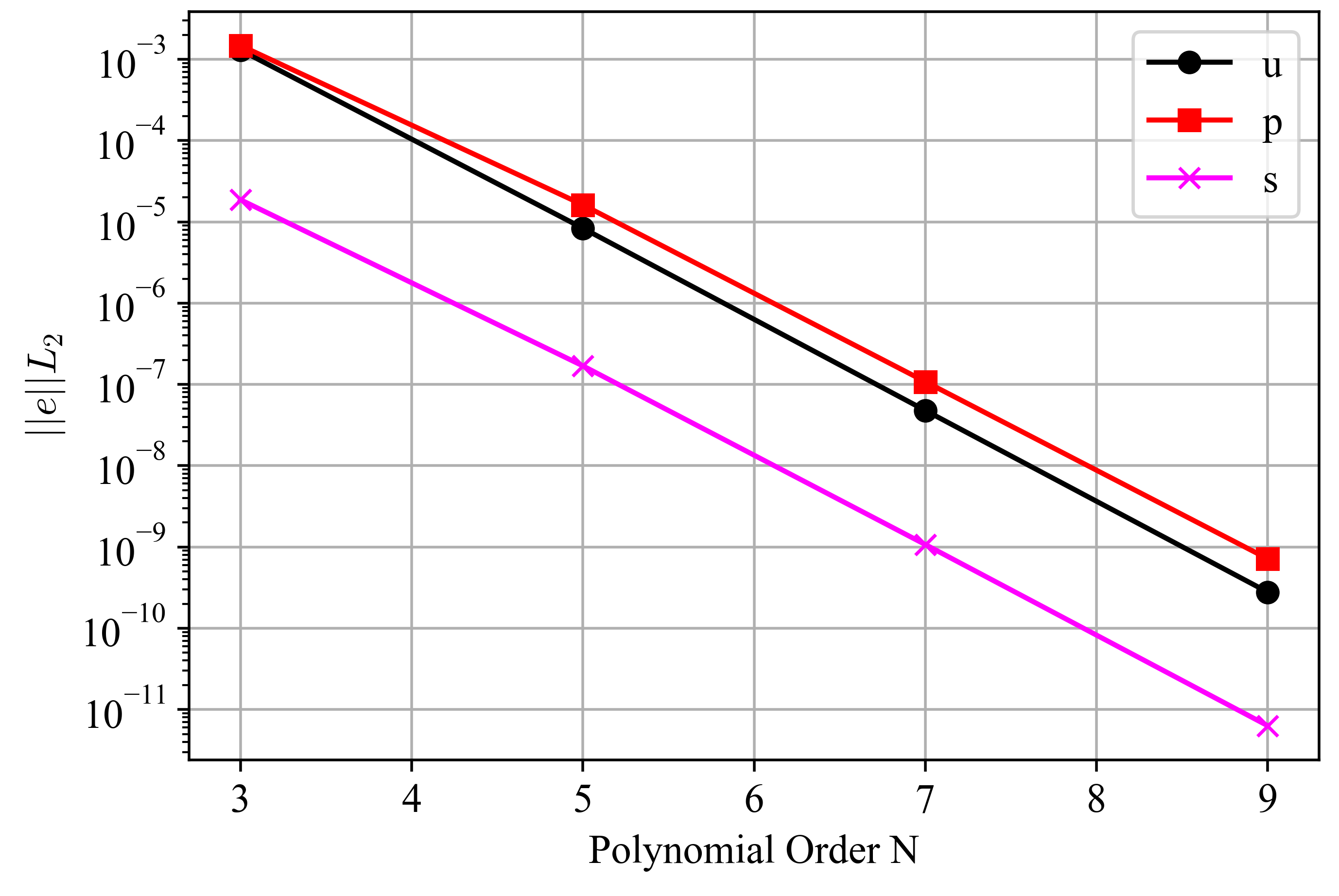
Figure 11: Spectral convergence under p refinement for the ethier case using solver mode 12; the routine regression test uses polynomial order nine.

Mode 14

This solver mode verifies:

Additive overlapping Schwarz pressure multigrid smoother.
Block velocity solver.
Characteristic subcycling.
Pressure projection.

The regression error is evaluated at $var element = document.getElementById("moose-equation-67e6cd05-b747-4b3d-bb1f-d84b2a150292");katex.render("t=0.06", element, {displayMode:false,throwOnError:false});$ . Figure 12 shows the corresponding $var element = document.getElementById("moose-equation-c45ddd24-ac3f-4970-b03a-90fb62f3dade");katex.render("p", element, {displayMode:false,throwOnError:false});$ -refinement study.

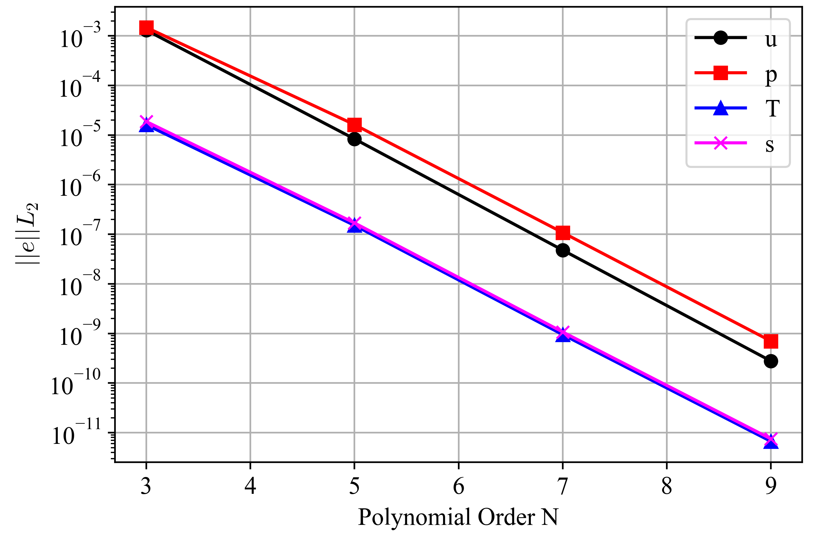
Spectral convergence of the Ethier solution errors using solver mode 14

Figure 12: Spectral convergence under p refinement for the ethier case using solver mode 14; the routine regression test uses polynomial order nine.

References

C Ross Ethier and DA Steinman. Exact fully 3d navier–stokes solutions for benchmarking. International Journal for Numerical Methods in Fluids, 19(5):369–375, 1994.

BibTeX

@article{ethier1994exact,
    author = "Ethier, C Ross and Steinman, DA",
    title = "Exact fully 3D Navier--Stokes solutions for benchmarking",
    journal = "International Journal for Numerical Methods in Fluids",
    volume = "19",
    number = "5",
    pages = "369--375",
    year = "1994",
    publisher = "Wiley Online Library"
}

RIS

TY  - JOUR
AU  - Ethier, C Ross
AU  - Steinman, DA
TI  - Exact fully 3D Navier–Stokes solutions for benchmarking
JO  - International Journal for Numerical Methods in Fluids
PY  - 1994
VL  - 19
IS  - 5
PB  - Wiley Online Library
SP  - 369
EP  - 375
ER  -

Plain Text

C Ross Ethier and DA Steinman. Exact fully 3d navier–stokes solutions for benchmarking. International Journal for Numerical Methods in Fluids, 19(5):369–375, 1994.

Computational domain
Analytical solution
Verification criteria
Mode 2
Mode 3
Mode 4
Mode 5
Mode 6
Mode 7
Mode 8
Mode 9
Mode 10
Mode 11
Mode 12
Mode 14
References