SFR Fuel Assembly
In this tutorial, you will learn how to:
Build a Cardinal model starting from simpler models for each individual physics
Omit portions of the OpenMC domain from multiphysics feedback
Couple OpenMC via temperature, density, and heat source feedback to the MOOSE heat conduction and subchannel modules
To access this tutorial,
cd cardinal/tutorials/openmc_subchannel
!alert! tip This tutorial was the basis for the IAEA/ICTP workshop held in Trieste in September 2025. For video recordings, please see the OpenMC, MOOSE, and Cardinal videos here. This Cardinal tutorial builds upon the OpenMC and MOOSE sections of the workshop.
The main focus of this tutorial is to teach you how to build a multiphysics simulation step by step. We first build the "single-physics" inputs for OpenMC, MOOSE heat conduction, and MOOSE subchannel using placeholder values for various source terms/boundary conditions. Then, we extend from these files to a full 3-physics coupled case.
Geometry
This model consists of the active region of the Chinese Experimental Fast Reactor (CEFR) fuel assembly. The relevant dimensions are summarized in Table 1. The geometry consists of annular UO fuel pins within a triangular lattice and enclosed in a duct. Sodium coolant is present outside the cladding.
Table 1: Geometric specifications for the SFR fuel assembly
| Parameter | Value (cm) |
|---|---|
| Fuel pellet outer diameter | 0.52 |
| Fuel pellet inner diameter | 0.16 |
| Fuel pin pitch | 0.695 |
| Clad inner diameter | 0.54 |
| Clad outer diameter | 0.6 |
| Height of active region | 45.0 |
| Assembly pitch | 6.1 |
| Duct inner flat-to-flat | 5.66 |
| Duct outer flat-to-flat | 5.9 |
The total core power of 65 MWth is assumed uniformly distributed among the 79 fuel bundles, so that the power of one fuel bundle will be normalized to 0.822 MWth.
In this tutorial, we will only solve for the multiphysics feedback in the interior-bundle region, i.e. for the sodium and fuel pins inside the duct. The thermal-fluid solution in the duct and inter-wrapper space (sodium outside the duct) will not be performed in order to illustrate how an OpenMC model (which does contain these regions) can be coupled to physics feedback over a subset of its domain. This simplification taken in this tutorial is not a limitation of any of the physics solvers and is only performed for illustration of a general notion often taken when building multiphysics models (i.e. usually, not all physics are solved over all parts of the domain). For instance, it is commonplace to omit the thermal-fluid solution in above-core regions like axial reflectors because temperature/density changes in these regions have only a small impact on the neutronics feedback (but these domains have to at least exist in the neutronics model or the leakage will be very wrong). Any uncoupled regions in OpenMC simply remain at the initial temperatures and densities in the OpenMC XML files.
The overall approach to build this three-physics coupled model will progress by first: 1. Building single-physics models for MOOSE heat conduction, OpenMC neutronics, and MOOSE subchannel with placeholder values for the boundary conditions and source terms required to couple the 3 physics together 2. Couple OpenMC and heat conduction in the solids 3. Couple OpenMC, heat conduction, and subchannel in the solids and fluids
Our eventual goal will be to accomplish the following multiphysics coupling shown in Figure 1 (this is step 3 above). Red arrows indicate those data transfers that Cardinal performs, while black arrows indicate Transfers we will use directly from the MOOSE framework. The mesh shown in the center of the image is the mesh in the main app's input, and will be the central landing/retrieval point for the coupling data passed between each of the three coupled solvers.
](../media/full_coupling.png)
Figure 1: Multiphysics data transfers we will require to couple OpenMC, heat conduction, and subchannel models of the within-duct region of an SFR
Before we progress to this more complicated model, we will first build individual models of each solver, with all incoming data transfers set to be placeholder values. Figure 2 shows each of the single-physics models we will build – we will not pass data to/from the centralized transfer mesh at this point, but will simply run each code and demonstrate how to set placeholder values for the data received by that application. Figure 2 represents step 1 above.
![Three single-physics models we will build to gradually progress to [full_coupling]](../media/single_coupling.png)
Figure 2: Three single-physics models we will build to gradually progress to Figure 1
Step 2 will then couple OpenMC to MOOSE heat conduction, with transfers shown in Figure 3. This will allow us to describe MultiApps and Transfers with just two of the physics solvers. Then, we will be ready to progress to the fully coupled case, Step 3, shown in Figure 1.

Figure 3: Progression to couple two codes together
Step 1: Single-Physics Uncoupled Models
Heat Conduction Model
First, we will create a heat conduction model for the fuel pins without any multiphysics feedback to OpenMC or the MOOSE subchannel module. To begin, we build a mesh of the fuel pins using MOOSE's reactor module for mesh-building. This mesh is built by first creating a mesh of a single fuel pin, then packing that pin into a hexagonal lattice, and finally by extruding this 2-D mesh into 3-D.
!include ../common.i

[Mesh]
  [pin]
    type = PolygonConcentricCircleMeshGenerator
    num_sides = 6
    ring_radii = '${fparse 1e-2*hole_diameter/2} ${fparse 1e-2*pellet_diameter/2} ${fparse 1e-2*inner_clad_diameter/2} ${fparse 1e-2*outer_clad_diameter/2}'
    ring_intervals = '1 5 1 1'
    num_sectors_per_side = '4 4 4 4 4 4'
    polygon_size = ${fparse 0.5 * pin_pitch * 1e-2}

    ring_block_ids = '0 1 0 2'
    ring_block_names = 'helium fuel helium clad'
    background_block_ids = '3'
    background_block_names = 'sodium'
    quad_center_elements = true
  []
  [assembly]
    type = PatternedHexMeshGenerator
    inputs = 'pin'
    pattern = '0 0 0 0 0;
              0 0 0 0 0 0;
             0 0 0 0 0 0 0;
            0 0 0 0 0 0 0 0;
           0 0 0 0 0 0 0 0 0;
            0 0 0 0 0 0 0 0;
             0 0 0 0 0 0 0;
              0 0 0 0 0 0;
               0 0 0 0 0'
    hexagon_size = ${fparse duct_inner_flat_to_flat * 1e-2/2}
    background_block_id = '3'
    background_block_name = 'sodium'
    rotate_angle = 60
  []
  [extrude]
    type = AdvancedExtruderGenerator
    input = assembly
    direction = '0 0 1'
    num_layers = '${n_layers}'
    heights = '${fparse height * 1e-2}'
  []
[]
To generate the mesh as a file, run the input file in mesh generation mode:
cardinal-opt -i mesh.i --mesh-only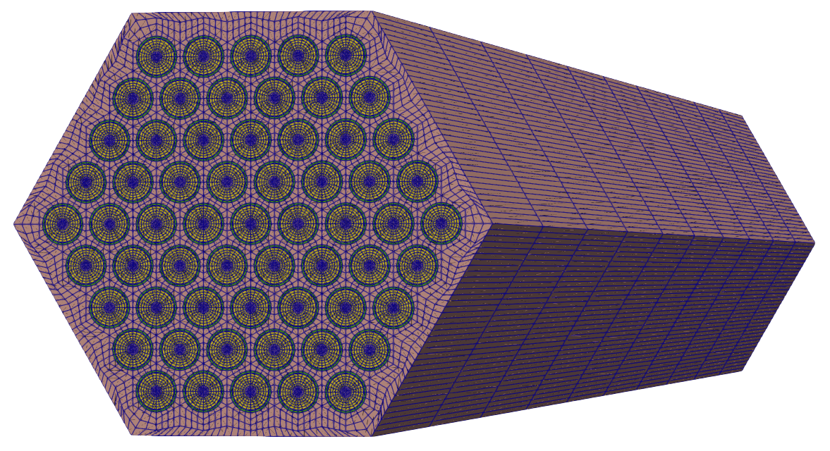
Figure 4: Mesh created by mesh.i
MOOSE mesh generators will often automatically set IDs to the sidesets in the model; in order to apply our pin surface temperature boundary condition, we need to know the ID of this sideset. This can be determined by reading the documentation for the various objects in the [Mesh] block, or by visually inspecting the model in Paraview. From Paraview's sideset panel, we can individually turn sidesets on/off, until we find that sideset 7 is the pin surface.
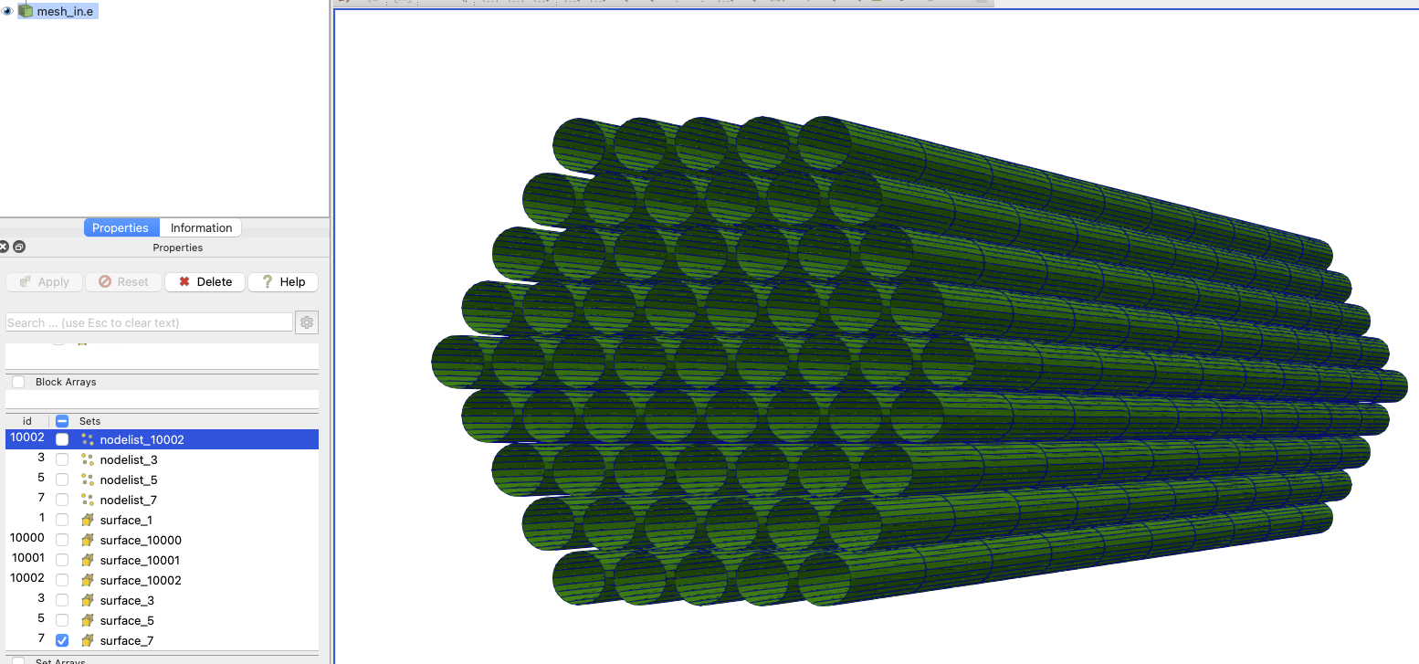
Figure 5: Paraview sideset viewer panel can be used to turn sideset views on/off until we find the number of the sideset representing the pin outer surface
Now that we have a mesh, we can create an input file to model heat conduction in the solid regions, without any multiphysics coupling. These files are located in the heat_conduction sub-folder. The first thing we need to do is actually modify the mesh we just made - you'll notice that this mesh contains the region pertaining to fluid, which we actually don't need for the heat conduction solve. This operation is shown by loading the mesh from the file and then applying another modification to it.
[Mesh<<<{"href": "../syntax/Mesh/index.html"}>>>]
  [file]
    type = FileMeshGenerator<<<{"description": "Read a mesh from a file.", "href": "../source/meshgenerators/FileMeshGenerator.html"}>>>
    file<<<{"description": "The filename to read."}>>> = ../meshes/mesh_in.e
  []
  [delete_coolant]
    type = BlockDeletionGenerator<<<{"description": "Mesh generator which removes elements from the specified subdomains", "href": "../source/meshgenerators/BlockDeletionGenerator.html"}>>>
    input<<<{"description": "The mesh we want to modify"}>>> = file
    block<<<{"description": "The list of blocks to be processed (deleted or kept)"}>>> = 'sodium'
  []
[]Next, we define the variables and governing equations for the heat conduction physics. We will be solving for temperature, so we first declare a variable named T. Then, we add two kernels, one to represent the diffusive kernel and the second to represent a volumetric heat source. This heat source will be provided by a coupled variable named heat_source and only exists on block 1, the fuel. The HeatConduction kernel requires specification of a material property named thermal_conductivity, for which we use three GenericConstantMaterial objects, to set unique values for on each subdomain in the mesh.
[Variables<<<{"href": "../syntax/Variables/index.html"}>>>]
  [T]
  []
[]

[Kernels<<<{"href": "../syntax/Kernels/index.html"}>>>]
  [heat_conduction]
    type = HeatConduction<<<{"description": "Diffusive heat conduction term $-\\nabla\\cdot(k\\nabla T)$ of the thermal energy conservation equation", "href": "../source/kernels/HeatConduction.html"}>>>
    variable<<<{"description": "The name of the variable that this residual object operates on"}>>> = T
  []
  [heat_source_fuel]
    type = CoupledForce<<<{"description": "Implements a source term proportional to the value of a coupled variable. Weak form: $(\\psi_i, -\\sigma v)$.", "href": "../source/kernels/CoupledForce.html"}>>>
    variable<<<{"description": "The name of the variable that this residual object operates on"}>>> = T
    v<<<{"description": "The coupled variable which provides the force"}>>> = heat_source
    block<<<{"description": "The list of blocks (ids or names) that this object will be applied"}>>> = 'fuel'
  []
[]

[Materials<<<{"href": "../syntax/Materials/index.html"}>>>]
   [k_helium]
    type = GenericConstantMaterial<<<{"description": "Declares material properties based on names and values prescribed by input parameters.", "href": "../source/materials/GenericConstantMaterial.html"}>>>
    prop_names<<<{"description": "The names of the properties this material will have"}>>> = 'thermal_conductivity'
    prop_values<<<{"description": "The values associated with the named properties"}>>> = '1.5'
    block<<<{"description": "The list of blocks (ids or names) that this object will be applied"}>>> = 'helium'
  []
   [k_fuel]
    type = GenericConstantMaterial<<<{"description": "Declares material properties based on names and values prescribed by input parameters.", "href": "../source/materials/GenericConstantMaterial.html"}>>>
    prop_names<<<{"description": "The names of the properties this material will have"}>>> = 'thermal_conductivity'
    prop_values<<<{"description": "The values associated with the named properties"}>>> = '2.0'
    block<<<{"description": "The list of blocks (ids or names) that this object will be applied"}>>> = 'fuel'
  []
   [k_clad]
    type = GenericConstantMaterial<<<{"description": "Declares material properties based on names and values prescribed by input parameters.", "href": "../source/materials/GenericConstantMaterial.html"}>>>
    prop_names<<<{"description": "The names of the properties this material will have"}>>> = 'thermal_conductivity'
    prop_values<<<{"description": "The values associated with the named properties"}>>> = '10.0'
    block<<<{"description": "The list of blocks (ids or names) that this object will be applied"}>>> = 'clad'
  []
[]Next, we define auxiliary variables for the fields involved in the coupling - T_wall will be used for the pin outer surface temperature (an input to the conduction model), heat_source will be used for the volumetric heating term (an input to the conduction model), and q_prime will be used for the linear heating rate (an output from the conduction model). For T_wall and heat_source, we set a simple initial condition of a constant value. The choice of 1e8 for the power density is arbitrary here, as we're simply trying to build one of our input files for a later multiphysics run where this information will come from OpenMC. Then, we apply a Dirichlet boundary condition, MatchedValueBC, to the pin outer surface.
[BCs<<<{"href": "../syntax/BCs/index.html"}>>>]
  [cladding_outer_bc]
    type = MatchedValueBC<<<{"description": "Implements a NodalBC which equates two different Variables' values on a specified boundary.", "href": "../source/bcs/MatchedValueBC.html"}>>>
    variable<<<{"description": "The name of the variable that this residual object operates on"}>>> = T
    v<<<{"description": "The variable whose value we are to match."}>>> = T_wall
    boundary<<<{"description": "The list of boundary IDs from the mesh where this object applies"}>>> = '7'
  []
[]For the linear heating rate (W/m), we use a NearestPointLayeredIntegral to compute an integral in the direction of the heat_source variable, individually for each fuel pin. This user object is then applied to fill the q_pime auxiliary variable with the SpatialUserObjectAux.
[AuxKernels<<<{"href": "../syntax/AuxKernels/index.html"}>>>]
  [q_prime]
    type = SpatialUserObjectAux<<<{"description": "Populates an auxiliary variable with a spatial value returned from a UserObject spatialValue method.", "href": "../source/auxkernels/SpatialUserObjectAux.html"}>>>
    variable<<<{"description": "The name of the variable that this object applies to"}>>> = q_prime
    user_object<<<{"description": "The UserObject UserObject to get values from.  Note that the UserObject _must_ implement the spatialValue() virtual function!"}>>> = q_prime_uo
    block<<<{"description": "The list of blocks (ids or names) that this object will be applied"}>>> = 'fuel'
  []
[]

[UserObjects<<<{"href": "../syntax/UserObjects/index.html"}>>>]
  [q_prime_uo]
    type = NearestPointLayeredIntegral<<<{"description": "Computes integrals of a variable storing partial sums for the specified number of intervals in a direction (x,y,z). Given a list of points this object computes the layered integral closest to each one of those points.", "href": "../source/userobjects/NearestPointLayeredIntegral.html"}>>>
    variable<<<{"description": "The name of the variable that this object operates on"}>>> = heat_source
    block<<<{"description": "The list of block ids (SubdomainID) that this object will be applied"}>>> = 'fuel'
    direction<<<{"description": "The direction of the layers."}>>> = z
    points_file<<<{"description": "A filename that should be looked in for points. Each set of 3 values in that file will represent a Point. This and 'points' cannot be both supplied."}>>> = '../pin_centers.txt'
    num_layers<<<{"description": "The number of layers."}>>> = ${n_layers}
  []
[]Finally, we select a Steady executioner and write outputs to exodus.
[Executioner<<<{"href": "../syntax/Executioner/index.html"}>>>]
  type = Steady
[]

[Outputs<<<{"href": "../syntax/Outputs/index.html"}>>>]
  exodus<<<{"description": "Output the results using the default settings for Exodus output."}>>> = true
[]We are now ready to run this model; for example, with 2 MPI ranks and 2 threads per rank,
mpiexec -np 2 cardinal-opt -i conduction.i --n-threads=2
We create an output file named conduction_out.e, which we can open in Paraview and view the solid temperature (left) and linear heat rate (right). The linear heat rate is constant because is constant.
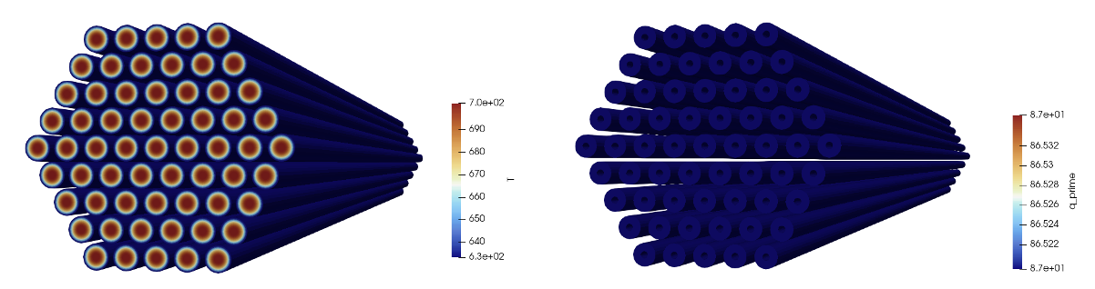
Figure 6: Solid temperature (left) and axial heat rate (right) computed by MOOSE heat conduction model with placeholder values for the pin surface temperature (constant) and power density (constant).
OpenMC Model
The OpenMC model is built using CSG, which are cells created from regions of space formed by half-spaces of various common surfaces. OpenMC's Python API is used to create the pincell model with the script shown below within the openmc folder. First, we define materials and create the geometry. We add create a universe representing a fuel pin, and then repeat that universe inside of a 3-D HexLattice, where the axial layers in the lattice create additional cells in the axial direction necessary to apply temperature and density feedback with a spatial distribution. The OpenMC model also contains the duct and sodium interassembly space; these regions will not be coupled to feedback from MOOSE, so we omit discretizing them in the axial direction for simplicity.
The OpenMC geometry as produced via plots is shown in Figure 7.
import openmc
import openmc.lib
import numpy as np
from matplotlib import pyplot as plt
import math

import os
import sys
script_dir = os.path.dirname(__file__)
sys.path.append(script_dir)
import common as specs

# This is a simplified OpenMC model of a CEFR fuel subassembly; for this multiphysics
# tutorial, we focus only on the active region, with a height of 45 cm
# (just out of simplicity and to make the training more tractable for the time allotted).

model = openmc.Model()

# --- Create materials

# UO2 for fuel
UO2 = openmc.Material(name="UO2")
UO2.set_density('sum')
UO2.add_nuclide('U235',1.49981E-02,'ao')
UO2.add_nuclide('U238',8.26381E-03,'ao')
UO2.add_nuclide('O16', 4.69512E-02,'ao')

# 15-15Ti stainless steel for the cladding
SS = openmc.Material(name="15-15Ti")
SS.set_density('atom/b-cm',density=8.49843E-02)
SS.add_nuclide('Fe54' ,3.18736E-03 )
SS.add_nuclide('Fe56' ,5.00347E-02 )
SS.add_nuclide('Fe57' ,1.15552E-03 )
SS.add_nuclide('Fe58' ,1.53779E-04 )
SS.add_nuclide('Cr50' ,6.43727E-04 )
SS.add_nuclide('Cr52' ,1.24136E-02 )
SS.add_nuclide('Cr53' ,1.40761E-03 )
SS.add_nuclide('Cr54' ,3.50383E-04 )
SS.add_nuclide('Ni58' ,8.11014E-03 )
SS.add_nuclide('Ni60' ,3.12399E-03 )
SS.add_nuclide('Ni61' ,1.35798E-04 )
SS.add_nuclide('Ni62' ,4.32997E-04 )
SS.add_nuclide('Ni64' ,1.10257E-04 )
SS.add_nuclide('Mo92' ,1.57916E-04 )
SS.add_nuclide('Mo94' ,9.94445E-05 )
SS.add_nuclide('Mo95' ,1.72153E-04 )
SS.add_nuclide('Mo96' ,1.81174E-04 )
SS.add_nuclide('Mo97' ,1.04335E-04 )
SS.add_nuclide('Mo98' ,2.65077E-04 )
SS.add_nuclide('Mo100',1.06726E-04 )
SS.add_nuclide('Mn55' ,1.29433E-03 )
SS.add_nuclide('C0'   ,2.37026E-04 )
SS.add_nuclide('Ti46' ,2.85966E-05 )
SS.add_nuclide('Ti47' ,2.57889E-05 )
SS.add_nuclide('Ti48' ,2.55532E-04 )
SS.add_nuclide('Ti49' ,1.87524E-05 )
SS.add_nuclide('Ti50' ,1.79552E-05 )
SS.add_nuclide('Si28' ,7.00451E-04 )
SS.add_nuclide('Si29' ,3.55834E-05 )
SS.add_nuclide('Si30' ,2.34843E-05 )

# Ti316 stainless steel for the duct
Ti316 = openmc.Material(name="Ti36")
Ti316.set_density('atom/b-cm',density=8.54309E-02)
Ti316.add_nuclide('Fe54' ,3.23855E-03)
Ti316.add_nuclide('Fe56' ,5.08384E-02)
Ti316.add_nuclide('Fe57' ,1.17408E-03)
Ti316.add_nuclide('Fe58' ,1.56248E-04)
Ti316.add_nuclide('Cr50' ,6.74283E-04)
Ti316.add_nuclide('Cr52' ,1.30029E-02)
Ti316.add_nuclide('Cr53' ,1.47442E-03)
Ti316.add_nuclide('Cr54' ,3.67015E-04)
Ti316.add_nuclide('Ni58' ,6.88162E-03)
Ti316.add_nuclide('Ni60' ,2.65077E-03)
Ti316.add_nuclide('Ni61' ,1.15228E-04)
Ti316.add_nuclide('Ni62' ,3.67407E-04)
Ti316.add_nuclide('Ni64' ,9.35550E-05)
Ti316.add_nuclide('Mo92' ,1.79675E-04)
Ti316.add_nuclide('Mo94' ,1.13147E-04)
Ti316.add_nuclide('Mo95' ,1.95874E-04)
Ti316.add_nuclide('Mo96' ,2.06138E-04)
Ti316.add_nuclide('Mo97' ,1.18712E-04)
Ti316.add_nuclide('Mo98' ,3.01602E-04)
Ti316.add_nuclide('Mo100',1.21432E-04)
Ti316.add_nuclide('Mn55' ,1.51194E-03)
Ti316.add_nuclide('C0'   ,2.37324E-04)
Ti316.add_nuclide('Ti46' ,3.27229E-05)
Ti316.add_nuclide('Ti47' ,2.95101E-05)
Ti316.add_nuclide('Ti48' ,2.92403E-04)
Ti316.add_nuclide('Ti49' ,2.14583E-05)
Ti316.add_nuclide('Ti50' ,2.05460E-05)
Ti316.add_nuclide('Si28' ,9.35106E-04)
Ti316.add_nuclide('Si29' ,4.75041E-05)
Ti316.add_nuclide('Si30' ,3.13517E-05)

# sodium for the coolant
sodium = openmc.Material(name="sodium")
sodium.set_density('sum')
sodium.add_nuclide('Na23',2.33599E-02)

# helium for the central hole in the fuel pin
He = openmc.Material(name="helium")
He.set_density('sum')
He.add_nuclide('He4',1.00000E-11)

# register the materials with the model object
model.materials = openmc.Materials([UO2, SS, Ti316, He, sodium])

# --- Define the geometry

# Define the surfaces needed for a fuel pin
helium_hole_surface = openmc.ZCylinder(x0=0, y0=0, r=specs.hole_diameter/2.0)
fuel_surface        = openmc.ZCylinder(x0=0, y0=0, r=specs.pellet_diameter/2.0)
clad_inner_surface  = openmc.ZCylinder(x0=0, y0=0, r=specs.inner_clad_diameter/2.0)
clad_outer_surface  = openmc.ZCylinder(x0=0, y0=0, r=specs.outer_clad_diameter/2.0)

# Define the surfaces needed for the various hexagons enclosing the assembly
hex_WR_IN    = openmc.model.HexagonalPrism(orientation='x', origin=(0.0, 0.0), edge_length=specs.duct_inner_flat_to_flat/math.sqrt(3))
hex_WR_OU    = openmc.model.HexagonalPrism(orientation='x', origin=(0.0, 0.0), edge_length=specs.duct_outer_flat_to_flat/math.sqrt(3.))
hex_SA_PITCH = openmc.model.HexagonalPrism(orientation='x', origin=(0.0, 0.0), edge_length=specs.assembly_pitch/math.sqrt(3.), boundary_type='reflective')

# define axial surfaces which will bound the active fissile region
lower = openmc.ZPlane(z0=0.0, boundary_type='vacuum')
upper = openmc.ZPlane(z0=specs.height, boundary_type='vacuum')

# create the cells in a fuel pin
helium_hole    = openmc.Cell(fill=He,     region=-helium_hole_surface)
fuel_annulus   = openmc.Cell(fill=UO2,    region=+helium_hole_surface & -fuel_surface)
helium_gap     = openmc.Cell(fill=He,     region=+fuel_surface & -clad_inner_surface)
ss_clad        = openmc.Cell(fill=SS,     region=+clad_inner_surface & -clad_outer_surface)
sodium_annulus = openmc.Cell(fill=sodium, region=+clad_outer_surface)

fuel_pin_universe = openmc.Universe(cells=[helium_hole, fuel_annulus, helium_gap, ss_clad, sodium_annulus])

# pure sodium universe
sodium_universe = openmc.Universe(cells=[openmc.Cell(fill=sodium)])

# create a lattice for a fuel assembly, consisting of 61 fuel pins
axial_pitch = specs.height / specs.n_layers
fuel_pin_lattice = openmc.HexLattice()
fuel_pin_lattice.orientation = 'x'
fuel_pin_lattice.center = [0., 0., specs.height/2]
fuel_pin_lattice.pitch  = [specs.pin_pitch, axial_pitch]

each_layer = [[sodium_universe]*30, [fuel_pin_universe]*24, [fuel_pin_universe]*18, [fuel_pin_universe]*12, [fuel_pin_universe]*6, [fuel_pin_universe]]
axial = []
for i in range(specs.n_layers):
  axial.append(each_layer)

fuel_pin_lattice.universes = axial

# put that fuel pin lattice inside a hexagon boundary, then add additional hexagons
# to represent the duct. For each, place inside the axial extents
layer = +lower & -upper
fuel_hex_cell = openmc.Cell(region=-hex_WR_IN & layer, fill=fuel_pin_lattice)
duct_cell = openmc.Cell(region=-hex_WR_OU & +hex_WR_IN & layer, fill=Ti316)
sodium_cell = openmc.Cell(region=+hex_WR_OU & -hex_SA_PITCH & layer, fill=sodium)

root = openmc.Universe(cells=[fuel_hex_cell, duct_cell, sodium_cell])
model.geometry = openmc.Geometry(root)

###############################################################################
#                   Exporting to OpenMC settings.xml file
###############################################################################

# Instantiate a Settings object, set all runtime parameters, and export to XML. Note
# that the choices for batches and particles are VERY low, and are only selected as
# these choices to get a fast-running model
model.settings.batches   = 120
model.settings.inactive  = 20
model.settings.particles = 1000

model.settings.ptables   = True
model.settings.temperature['method']='interpolation'
model.settings.temperature['range'] = (300.0, 3000.0)
model.settings.temperature['default'] = 0.5 * (specs.inlet_temperature + specs.outlet_temperature)

# Create an initial uniform spatial source distribution over fissionable zones
l = specs.assembly_pitch
bounds = [-l, -l, 0.0, l, l, specs.height]
uniform_dist = openmc.stats.Box(bounds[:3], bounds[3:])
model.settings.source = openmc.source.IndependentSource(space=uniform_dist, constraints={'fissionable' : True})

# Create some plots for visualization
xy          = openmc.Plot()
xy.filename = 'xy'
xy.width    = (8, 8)
xy.basis    = 'xy'
xy.origin   = (0.0, 0.0, 0.5*specs.height)
xy.pixels   = (2000, 2000)
xy.color_by = 'material'

xz          = openmc.Plot()
xz.filename = 'xz'
xz.width    = (l, specs.height*1.5)
xz.basis    = 'xz'
xz.origin   = (0.0, 0.0, 0.5*specs.height)
xz.pixels   = (2000, 2000)
xz.color_by = 'material'

xy_cell          = openmc.Plot()
xy_cell.filename = 'xy_cell'
xy_cell.width    = (8, 8)
xy_cell.basis    = 'xy'
xy_cell.origin   = (0.0, 0.0, 0.5*specs.height)
xy_cell.pixels   = (2000, 2000)
xy_cell.color_by = 'cell'

xz_cell          = openmc.Plot()
xz_cell.filename = 'xz_cell'
xz_cell.width    = (l, specs.height*1.5)
xz_cell.basis    = 'xz'
xz_cell.origin   = (0.0, 0.0, 0.5*specs.height)
xz_cell.pixels   = (2000, 2000)
xz_cell.color_by = 'cell'

model.plots = openmc.Plots([xy, xz, xy_cell, xz_cell])

model.export_to_model_xml()

Figure 7: OpenMC geometry colored by cell ID (left) and material (right) shown on the - plane
The top and bottom of the domain are vacuum boundaries, while the six lateral faces are reflective. Because we fill the fuel_pin_universe within the entries in the fuel_pin_lattice, and we fill the fuel_pin_lattice inside the hex_WR_IN surface, applying individual temperatures to each pin and axial layer will require us to set lowest_cell_level = 2.
To generate the XML files needed to run OpenMC, you can run the following:
python model.py
or simply use the XML files checked in to the tutorials/openmc_subchannel/openmc directory.
Now, to run OpenMC via Cardinal we need to create a thin wrapper input file, shown below. We begin by loading the mesh generated earlier; this mesh is not actually used by OpenMC, but is where OpenMC will read temperatures/densities from, and to where it will write tallies.
[Mesh<<<{"href": "../syntax/Mesh/index.html"}>>>]
  [file]
    type = FileMeshGenerator<<<{"description": "Read a mesh from a file.", "href": "../source/meshgenerators/FileMeshGenerator.html"}>>>
    file<<<{"description": "The filename to read."}>>> = ../meshes/mesh_in.e
  []
[]Next, we create a block which will override the typical finite element/volume MOOSE solve by running OpenMC. In this block, we specify the power level we want to normalize the tallies to (see here) for more information). Then, we indicate which subdomains in the mesh OpenMC will read temperature from and read density from. We only read densities for the fluid because any density changes in the solid would require movement of cell boundaries in order to preserve masses. Then, we finish by creating a tally over the OpenMC cells, which will automatically get written into an auxiliary variable named kappa_fission.
[Problem<<<{"href": "../syntax/Problem/index.html"}>>>]
  type = OpenMCCellAverageProblem
  power = ${power}
  lowest_cell_level = 2
  scaling = 100

  temperature_blocks = 'helium fuel clad sodium'
  density_blocks = 'sodium'

  [Tallies<<<{"href": "../syntax/Problem/Tallies/index.html"}>>>]
    [power]
      type = CellTally<<<{"description": "A class which implements distributed cell tallies.", "href": "../source/tallies/CellTally.html"}>>>
      score<<<{"description": "Score(s) to use in the OpenMC tallies. If not specified, defaults to 'kappa_fission'"}>>> = 'kappa_fission'
    []
  []
[]The other coupled codes will provide temperatures and densities to OpenMC, but for this single-physics model we first simply set placeholder values for the temperatures and densities to be read by OpenMC. We also create two auxiliary variables that will display on the mesh the actual cell temperatures and densities used in OpenMC; these can be used to confirm that data read from the mesh gets applied correctly to the OpenMC domain.
[ICs<<<{"href": "../syntax/Cardinal/ICs/index.html"}>>>]
  [temp]
    type = ConstantIC<<<{"description": "Sets a constant field value.", "href": "../source/ics/ConstantIC.html"}>>>
    variable<<<{"description": "The variable this initial condition is supposed to provide values for."}>>> = temp
    value<<<{"description": "The value to be set in IC"}>>> = ${inlet_temperature}
  []
  [density]
    type = ConstantIC<<<{"description": "Sets a constant field value.", "href": "../source/ics/ConstantIC.html"}>>>
    variable<<<{"description": "The variable this initial condition is supposed to provide values for."}>>> = density
    value<<<{"description": "The value to be set in IC"}>>> = ${fparse 1.00423e3 + -0.21390*inlet_temperature+-1.1046e-5*inlet_temperature^2}
  []
[]

[AuxVariables<<<{"href": "../syntax/AuxVariables/index.html"}>>>]
  [cell_temperature]
    family<<<{"description": "Specifies the family of FE shape functions to use for this variable"}>>> = MONOMIAL
    order<<<{"description": "Specifies the order of the FE shape function to use for this variable (additional orders not listed are allowed)"}>>> = CONSTANT
  []
  [cell_density]
    family<<<{"description": "Specifies the family of FE shape functions to use for this variable"}>>> = MONOMIAL
    order<<<{"description": "Specifies the order of the FE shape function to use for this variable (additional orders not listed are allowed)"}>>> = CONSTANT
  []
[]

[AuxKernels<<<{"href": "../syntax/AuxKernels/index.html"}>>>]
  [cell_temperature]
    type = CellTemperatureAux<<<{"description": "OpenMC cell temperature (K), mapped to each MOOSE element", "href": "../source/auxkernels/CellTemperatureAux.html"}>>>
    variable<<<{"description": "The name of the variable that this object applies to"}>>> = cell_temperature
  []
  [cell_density]
    type = CellDensityAux<<<{"description": "OpenMC fluid density (kg/m$^3$), mapped to each MOOSE element", "href": "../source/auxkernels/CellDensityAux.html"}>>>
    variable<<<{"description": "The name of the variable that this object applies to"}>>> = cell_density
  []
[]Finally, we specify a steady executioner and output results to exodus.
[Executioner<<<{"href": "../syntax/Executioner/index.html"}>>>]
  type = Steady
[]

[Outputs<<<{"href": "../syntax/Outputs/index.html"}>>>]
  exodus<<<{"description": "Output the results using the default settings for Exodus output."}>>> = true
[]To run the model,
cardinal-opt -i openmc.i
This will generate an output file, openmc_out.e, which we can use to visualize the tally. We note that we see 10 "layers" in the tally in the axial direction, because we've subdivided the OpenMC model into 10 unique cells in the axial direction.

Figure 8: OpenMC kappa-fission score mapped to the mesh
We can also inspect the cell_temperature and cell_density variables, and find that they reflect the temperatures/densities that OpenMC reads from the mesh.
Subchannel Model
The fluid thermal-fluid model is built using MOOSE's subchannel module. The subchannel module is quite a bit different from a typical MOOSE application, because the subchannel method is fundamentally different from the finite element/finite volume methods used elsewhere in MOOSE. The purpose of this tutorial is not to serve as training on the subchannel module, so we encourage you to explore the subchannel module examples for more information on how the subchannel solver works. Here, we will only quickly describe the subchannel input file.
A subchannel method does not use a typical unstructured mesh - rather, the geometry is represented in a regimented way as a pseudo 2-D geometry stored as internal data structures in the MOOSE subchannel module. We build a 1-D mesh for each subchannel and fuel pin, just as a retrieval/landing point to store data computed by subchannel (though it should be understood that the solution from subchannel does allow crossflows between subchannels, so it is 2-D solver and not a 1-D solver as the mesh might suggest).
[TriSubChannelMesh<<<{"href": "../syntax/TriSubChannelMesh/index.html"}>>>]
  [subchannel]
    type = SCMTriAssemblyMeshGenerator<<<{"description": "Creates a mesh of 1D subchannels and 1D pins in a triangular lattice arrangement", "href": "../source/meshgenerators/SCMTriAssemblyMeshGenerator.html"}>>>
    nrings<<<{"description": "Number of fuel-pin rings per assembly, counting the center pin as the first ring [-]"}>>> = 5
    n_cells<<<{"description": "The number of cells in the axial direction"}>>> = 100
    flat_to_flat<<<{"description": "Flat to flat distance for the hexagonal assembly [m]"}>>> = '${fparse duct_inner_flat_to_flat * 1e-2}'
    heated_length<<<{"description": "Heated length [m]"}>>> = '${fparse height * 1e-2}'
    pin_diameter<<<{"description": "Rod diameter [m]"}>>> = '${fparse outer_clad_diameter * 1e-2}'
    pitch<<<{"description": "Pitch [m]"}>>> = '${fparse pin_pitch * 1e-2}'
    dwire<<<{"description": "Wire diameter [m]"}>>> = '${fparse wire_diameter * 1e-2}'
    hwire<<<{"description": "Wire lead length [m]"}>>> = '${fparse wire_pitch * 1e-2}'
  []
[]One auxiliary variable is created for all aspects of the subchannel solution - including the solution fields temperature (T), mass flowrates per channel (mdot), and pressure (P). Additional auxiliary variables are used to store the geometry information per channel, such as the cross-sectional flow areas (S) and wetted perimeters (w_perim). This block will always be the same for all subchannel models. We set a constant placeholder value for the linear heating rate, q_prime in lieu of a value to be provided by the heat conduction model. Additional subchannel-specific initial conditions are needed for some of the internal variables in the subchannel model; for example, SCMTriFlowAreaIC calculates the subchannel cross-sectional flow areas for the S auxiliary variable.
!include ../common.i

# compute the inlet mass flux required to get a bulk temperature rise of 160 K,
# for the imposed power of ${power}. We evaluate the specific heat at the average
# of the inlet and outlet temperatures using a correlation.
temperature = ${fparse 0.5 * (outlet_temperature + inlet_temperature)}
dt = ${fparse 2503.3 - temperature}
Cp = ${fparse 7.3898e5 / dt / dt + 3.154e5 / dt + 1.1340e3 + -2.2153e-1 * dt + 1.1156e-4 * dt * dt}
total_mdot = ${fparse power / Cp / (outlet_temperature - inlet_temperature)}

# compute the mass flux by dividing the mass flowrate by the flow area
flow_area = ${fparse sqrt(3)/2 * (duct_inner_flat_to_flat*1e-2)^2 - 61*pi*(outer_clad_diameter*1e-2)^2/4}

mass_flux_in = ${fparse total_mdot / flow_area}

[TriSubChannelMesh]
  [subchannel]
    type = SCMTriAssemblyMeshGenerator
    nrings = 5
    n_cells = 100
    flat_to_flat = ${fparse duct_inner_flat_to_flat * 1e-2}
    heated_length = ${fparse height * 1e-2}
    pin_diameter = ${fparse outer_clad_diameter * 1e-2}
    pitch = ${fparse pin_pitch * 1e-2}
    dwire = ${fparse wire_diameter * 1e-2}
    hwire = ${fparse wire_pitch * 1e-2}
  []
[]

[ICs]
  [T_IC]
    type = ConstantIC
    variable = T
    value = 500
  []
  [Dpin_IC]
    type = ConstantIC
    variable = Dpin
    value = ${fparse 1e-2 * outer_clad_diameter}
  []
  [q_prime_IC]
    type = ConstantIC
    variable = q_prime
    value = ${fparse power/61/(height*1e-2)}
  []
  [Viscosity_ic]
    type = ViscosityIC
    variable = mu
    p = ${P_out}
    T = T
    fp = sodium
  []
  [rho_ic]
    type = RhoFromPressureTemperatureIC
    variable = rho
    p = ${P_out}
    T = T
    fp = sodium
  []
  [h_ic]
    type = SpecificEnthalpyFromPressureTemperatureIC
    variable = h
    p = ${P_out}
    T = T
    fp = sodium
  []
[]
Next, we define the fluid properties and the problem solver settings. For instance, we set the tolerances for the pressure and temperature solves, and choices for staggering of the solution of the coupled equations for pressure, flow, and temperature. Two auxkernels are also used to apply the inlet conditions on temperature and flowrate.
[FluidProperties<<<{"href": "../syntax/FluidProperties/index.html"}>>>]
  [sodium]
    type = PBSodiumFluidProperties<<<{"description": "Class that provides the methods that realize the equations of state for Liquid Sodium", "href": "../source/fluidproperties/PBSodiumFluidProperties.html"}>>>
  []
[]

[SubChannel<<<{"href": "../syntax/SubChannel/index.html"}>>>]
  type = TriSubChannel1PhaseProblem
  fp = sodium
  n_blocks = 1
  P_out = ${P_out}
  compute_density = true
  compute_viscosity = true
  compute_power = true
  implicit = true
  segregated = false
  friction_closure = 'cheng_friction'
  mixing_closure = 'cheng_mixing'
  pin_HTC_closure = 'Dittus-Boelter'
  staggered_pressure = false
  P_tol = 1.0e-5
  T_tol = 1.0e-5
[]

[SCMClosures<<<{"href": "../syntax/SCMClosures/index.html"}>>>]
  [cheng_friction]
    type = SCMFrictionUpdatedChengTodreas<<<{"description": "Class that computes the axial friction factor using the updated Cheng Todreas correlations.", "href": "../source/scmclosures/SCMFrictionUpdatedChengTodreas.html"}>>>
  []
  [cheng_mixing]
    type = SCMMixingChengTodreas<<<{"description": "Class that models the turbulent mixing coefficient for wire-wrapped triangular assemblies using the Cheng Todreas correlations.", "href": "../source/scmclosures/SCMMixingChengTodreas.html"}>>>
  []
  [Dittus-Boelter]
    type = SCMHTCDittusBoelter<<<{"description": "Class that computes the convective heat transfer coefficient using the Dittus Boelter correlation.", "href": "../source/scmclosures/SCMHTCDittusBoelter.html"}>>>
  []
[]

[AuxKernels<<<{"href": "../syntax/AuxKernels/index.html"}>>>]
  [T_in_bc]
    type = ConstantAux<<<{"description": "Creates a constant field in the domain.", "href": "../source/auxkernels/ConstantAux.html"}>>>
    variable<<<{"description": "The name of the variable that this object applies to"}>>> = T
    boundary<<<{"description": "The list of boundaries (ids or names) from the mesh where this object applies"}>>> = inlet
    value<<<{"description": "Some constant value that can be read from the input file"}>>> = ${inlet_temperature}
    execute_on<<<{"description": "The list of flag(s) indicating when this object should be executed. For a description of each flag, see https://mooseframework.inl.gov/source/interfaces/SetupInterface.html."}>>> = 'timestep_begin'
  []
  [mdot_in_bc]
    type = SCMMassFlowRateAux<<<{"description": "Computes mass flow rate from specified mass flux and subchannel cross-sectional area. Can read either PostprocessorValue or Real", "href": "../source/auxkernels/SCMMassFlowRateAux.html"}>>>
    variable<<<{"description": "The name of the variable that this object applies to"}>>> = mdot
    boundary<<<{"description": "The list of boundaries (ids or names) from the mesh where this object applies"}>>> = inlet
    area<<<{"description": "Cross sectional area [m^2]"}>>> = S
    mass_flux<<<{"description": "The postprocessor or Real to use for the value of mass_flux"}>>> = ${mass_flux_in}
    execute_on<<<{"description": "The list of flag(s) indicating when this object should be executed. For a description of each flag, see https://mooseframework.inl.gov/source/interfaces/SetupInterface.html."}>>> = 'timestep_begin'
  []
[]To ensure the model is set up correctly, we can check the global energy conservation – the power deposited from the pins into the coolant should equal provided that no heat is lost through the lateral walls of the assembly (true for this problem setup), all changes to internal energy arise from sensible heat (i.e. no latent heat), the flow is steady-state, and the pressure work is negligible. We add postprocessors to compute the total power deposited in the subchannel model, as well as the bulk average inlet and outlet temperatures. The average specific heat is computed at the top of the input file with local parser syntax based on the correlation used for sodium.
[Postprocessors<<<{"href": "../syntax/Postprocessors/index.html"}>>>]
  [power]
    type = SCMPinPowerPostprocessor<<<{"description": "Calculates the total heat rate that goes into the coolant from all the heated fuel-pins based on aux variable q_prime", "href": "../source/postprocessors/SCMPinPowerPostprocessor.html"}>>>
  []
  [inlet_temp]
    type = SCMPlanarMean<<<{"description": "Calculates an mass-flow-rate averaged mean of the chosen variable on a z-plane at a user defined height over all subchannels", "href": "../source/postprocessors/SCMPlanarMean.html"}>>>
    variable<<<{"description": "Variable you want the mean of"}>>> = T
    height<<<{"description": "Axial location of plane [m]"}>>> = 0.0
  []
  [outlet_temp]
    type = SCMPlanarMean<<<{"description": "Calculates an mass-flow-rate averaged mean of the chosen variable on a z-plane at a user defined height over all subchannels", "href": "../source/postprocessors/SCMPlanarMean.html"}>>>
    variable<<<{"description": "Variable you want the mean of"}>>> = T
    height<<<{"description": "Axial location of plane [m]"}>>> = '${fparse height * 1e-2}'
  []
  [expected_dT]
    type = ParsedPostprocessor<<<{"description": "Computes a parsed expression with post-processors", "href": "../source/postprocessors/ParsedPostprocessor.html"}>>>
    expression<<<{"description": "function expression"}>>> = 'power/${total_mdot}/${Cp}'
    pp_names<<<{"description": "Post-processors arguments"}>>> = 'power'
  []
[]Finally, we specify a steady executioner and will output our results to exodus format. In order to visualize the subchannel solution in a domain which better represents the subchannel discretization, we pass a few of the subchannel solution variables to a sub-application in the viz.i file, which will simply render those variables into a format recognizable as subchannel discretization.
[Executioner<<<{"href": "../syntax/Executioner/index.html"}>>>]
  type = Steady
[]

[Outputs<<<{"href": "../syntax/Outputs/index.html"}>>>]
  exodus<<<{"description": "Output the results using the default settings for Exodus output."}>>> = true
[]

[MultiApps<<<{"href": "../syntax/MultiApps/index.html"}>>>]
  [viz]
    type = FullSolveMultiApp<<<{"description": "Performs a complete simulation during each execution.", "href": "../source/multiapps/FullSolveMultiApp.html"}>>>
    input_files<<<{"description": "The input file for each App.  If this parameter only contains one input file it will be used for all of the Apps.  When using 'positions_from_file' it is also admissable to provide one input_file per file."}>>> = 'viz.i'
    execute_on<<<{"description": "The list of flag(s) indicating when this object should be executed. For a description of each flag, see https://mooseframework.inl.gov/source/interfaces/SetupInterface.html."}>>> = 'timestep_end'
  []
[]

[Transfers<<<{"href": "../syntax/Transfers/index.html"}>>>]
  [transfer]
    type = SCMSolutionTransfer<<<{"description": "Transfers subchannel or pin solutions from a SubChannel mesh onto a visualization mesh.", "href": "../source/transfers/SCMSolutionTransfer.html"}>>>
    to_multi_app<<<{"description": "The name of the MultiApp to transfer the data to"}>>> = viz
    variable<<<{"description": "The auxiliary variables to transfer."}>>> = 'mdot P T rho S'
  []
[]The viz.i file does not solve any additional physics, but simply adds a 3-D mesh (not used for any solution) to visualize the subchannel solution.
!include ../common.i

[TriSubChannelMesh]
  [subchannel]
    type = SCMDetailedTriSubChannelMeshGenerator
    nrings = 5
    n_cells = 100
    flat_to_flat = ${fparse duct_inner_flat_to_flat * 1e-2}
    heated_length = ${fparse height * 1e-2}
    pin_diameter = ${fparse outer_clad_diameter * 1e-2}
    pitch = ${fparse pin_pitch * 1e-2}
  []
[]

[AuxVariables]
  [mdot]
    block = subchannel
  []
  [P]
    block = subchannel
  []
  [T]
    block = subchannel
  []
  [rho]
    block = subchannel
  []
  [S]
    block = subchannel
  []
[]

[Problem]
  type = NoSolveProblem
[]

[Outputs]
  exodus = true
[]

[Executioner]
  type = Steady
[]
We are now ready to run this model:
cardinal-opt -i subchannel.i
This will create two output files - subchannel_out.e which contains the subchannel solution, but shown on 1-D lines (this is just how subchannel stores its solution internally). The subchannel_out_viz0.e file shows the same data, but in a format representative of the subchannel discretization.

Figure 9: Subchannel solution for fluid temperature given a constant linear heating rate
We can confirm that this model conserves energy by comparing the value of the expected_dT postprocessor with the difference between the inlet_temp and outlet_temp postprocessors (the match is not perfect because we took the specific heat just at a single value, averaged over the bundle (in other words, we were not 100% precise in the expression used in expected_dT – energy is conserved if we did a more sophisticated integral of ).
Step 2: Two-Way Multiphysics Coupling
In this section, two of the codes are coupled together - OpenMC and MOOSE heat conduction in the solids. The following sub-sections describe these files, with the focus only on those aspects which are now different to couple two models together.
Heat Conduction Model
The only change required to the heat conduction model is that we add a postprocessor which will integrate the power density over the solid mesh to compute the received power from OpenMC - this is required in case the meshes differ between (i) where the tally is written by OpenMC vs. (ii) the mesh used to solve for heat conduction, so that energy conservation can be enforced.
[Postprocessors<<<{"href": "../syntax/Postprocessors/index.html"}>>>]
  [conduction_power_integral]
    type = ElementIntegralVariablePostprocessor<<<{"description": "Computes a volume integral of the specified variable", "href": "../source/postprocessors/ElementIntegralVariablePostprocessor.html"}>>>
    variable<<<{"description": "The name of the variable that this object operates on"}>>> = heat_source
    block<<<{"description": "The list of blocks (ids or names) that this object will be applied"}>>> = 'fuel'
    execute_on<<<{"description": "The list of flag(s) indicating when this object should be executed. For a description of each flag, see https://mooseframework.inl.gov/source/interfaces/SetupInterface.html."}>>> = 'transfer'
  []
[]We also require the heat conduction model to now use a Transient executioner, because we will be running the model multiple times (due to back and forth coupling with OpenMC).
[Executioner<<<{"href": "../syntax/Executioner/index.html"}>>>]
  type = Transient
[]Finally, to make the model a little bit more interesting, let's set the fluid temperature to a linear function from the inlet to the outlet (we will later use a subchannel model to actually compute this field). For this, we define a function with a linear depencence on height and spanning between the inlet and outlet temperatures, then apply it to the T_wall auxiliary variable.
[Functions<<<{"href": "../syntax/Functions/index.html"}>>>]
  [axial]
    type = ParsedFunction<<<{"description": "Function created by parsing a string", "href": "../source/functions/MooseParsedFunction.html"}>>>
    value = '${inlet_temperature}+z/${fparse height*1e-2}*(${outlet_temperature}-${inlet_temperature})'
  []
[][AuxKernels<<<{"href": "../syntax/AuxKernels/index.html"}>>>]
[q_prime]
type = SpatialUserObjectAux<<<{"description": "Populates an auxiliary variable with a spatial value returned from a UserObject spatialValue method.", "href": "../source/auxkernels/SpatialUserObjectAux.html"}>>>
variable<<<{"description": "The name of the variable that this object applies to"}>>> = q_prime
user_object<<<{"description": "The UserObject UserObject to get values from. Note that the UserObject _must_ implement the spatialValue() virtual function!"}>>> = q_prime_uo
block<<<{"description": "The list of blocks (ids or names) that this object will be applied"}>>> = 'fuel'
[]
[T_wall]
type = FunctionAux<<<{"description": "Auxiliary Kernel that creates and updates a field variable by sampling a function through space and time.", "href": "../source/auxkernels/FunctionAux.html"}>>>
variable<<<{"description": "The name of the variable that this object applies to"}>>> = T_wall
function<<<{"description": "The function to use as the value"}>>> = axial
[]
[]OpenMC Model
No changes are required to the XML files; we will simply add the MultiApps and Transfers to communicate data between OpenMC and the heat conduction model. We can select either OpenMC or MOOSE to be the main, controlling application - here, we select OpenMC.
The only changes we require to the OpenMC input file are to (i) switch to a Transient executioner and to add the MultiApps and Transfers blocks. We register a multiapp to solve the heat conduction physics. Then, we add two data transfers to represent the data received/computed by OpenMC to couple with heat conduction. These transfers will pass mesh-based data using a nearest-node transfer. First, OpenMC will pass the power distribution to the solid, making sure to conserve power by normalizing the received heat_source in the conduction.i file by the ratio of the power integral on the source and receiving mesh. The second transfer retrieves solid temperatures from the conduction model and applies them to the solid blocks in the mesh. By using a transient executioner, we can require the model to run for a fixed number of Picard iterations (5, in this example). Automated Picard convergence options, such as steady-state detection, are recommended for production calculations.
[Executioner<<<{"href": "../syntax/Executioner/index.html"}>>>]
  type = Transient
  num_steps = 5
[]

[Outputs<<<{"href": "../syntax/Outputs/index.html"}>>>]
  exodus<<<{"description": "Output the results using the default settings for Exodus output."}>>> = true
[]

[MultiApps<<<{"href": "../syntax/MultiApps/index.html"}>>>]
  [conduction]
    type = TransientMultiApp<<<{"description": "MultiApp for performing coupled simulations with the parent and sub-application both progressing in time.", "href": "../source/multiapps/TransientMultiApp.html"}>>>
    input_files<<<{"description": "The input file for each App.  If this parameter only contains one input file it will be used for all of the Apps.  When using 'positions_from_file' it is also admissable to provide one input_file per file."}>>> = 'conduction.i'
    sub_cycling<<<{"description": "Set to true to allow this MultiApp to take smaller timesteps than the rest of the simulation.  More than one timestep will be performed for each parent application timestep"}>>> = true
    execute_on<<<{"description": "The list of flag(s) indicating when this object should be executed. For a description of each flag, see https://mooseframework.inl.gov/source/interfaces/SetupInterface.html."}>>> = timestep_end
  []
[]

[Transfers<<<{"href": "../syntax/Transfers/index.html"}>>>]
  [power_to_conduction]
    type = MultiAppGeneralFieldNearestLocationTransfer<<<{"description": "Transfers field data at the MultiApp position by finding the value at the nearest neighbor(s) in the origin application.", "href": "../source/transfers/MultiAppGeneralFieldNearestLocationTransfer.html"}>>>
    to_multi_app<<<{"description": "The name of the MultiApp to transfer the data to"}>>> = conduction
    source_variable<<<{"description": "The variable to transfer from."}>>> = kappa_fission
    variable<<<{"description": "The auxiliary variable to store the transferred values in."}>>> = heat_source
    from_postprocessors_to_be_preserved<<<{"description": "The name of the Postprocessor in the from-app to evaluate an adjusting factor."}>>> = openmc_power_integral
    to_postprocessors_to_be_preserved<<<{"description": "The name of the Postprocessor in the to-app to evaluate an adjusting factor."}>>> = conduction_power_integral
  []
  [solid_temperature_from_conduction]
    type = MultiAppGeneralFieldNearestLocationTransfer<<<{"description": "Transfers field data at the MultiApp position by finding the value at the nearest neighbor(s) in the origin application.", "href": "../source/transfers/MultiAppGeneralFieldNearestLocationTransfer.html"}>>>
    from_multi_app<<<{"description": "The name of the MultiApp to receive data from"}>>> = conduction
    source_variable<<<{"description": "The variable to transfer from."}>>> = T
    variable<<<{"description": "The auxiliary variable to store the transferred values in."}>>> = temp
    to_blocks<<<{"description": "Subdomain restriction to transfer to, (defaults to all the target app domain)"}>>> = 'fuel clad helium'
  []
[]

[Postprocessors<<<{"href": "../syntax/Postprocessors/index.html"}>>>]
  [openmc_power_integral]
    type = ElementIntegralVariablePostprocessor<<<{"description": "Computes a volume integral of the specified variable", "href": "../source/postprocessors/ElementIntegralVariablePostprocessor.html"}>>>
    variable<<<{"description": "The name of the variable that this object operates on"}>>> = kappa_fission
    execute_on<<<{"description": "The list of flag(s) indicating when this object should be executed. For a description of each flag, see https://mooseframework.inl.gov/source/interfaces/SetupInterface.html."}>>> = 'transfer timestep_end'
  []
[]Running
We can now run the two-physics coupled model. For example, with 2 MPI ranks and 3 threads per rank,
mpiexec -np 3 cardinal-opt -i openmc.i
This will create two output files - openmc_out.e, which contains all the variables defined in the openmc.i file; and openmc_out_conduction0.e, which will contain all the variables defined in the conduction.i file. Inspecting the files, we can compare the cell_temperature in the openmc_out.e, which shows the actual temperatures applied to the OpenMC cells, against the continuous finite element temperature field solved by the heat conduction solver (T in openmc_out_conduction0.e). In Figure 10, a comparison between these two fields is shown on the axial midplane of the fuel (left). The continuous finite element conduction solution is shown on the right.
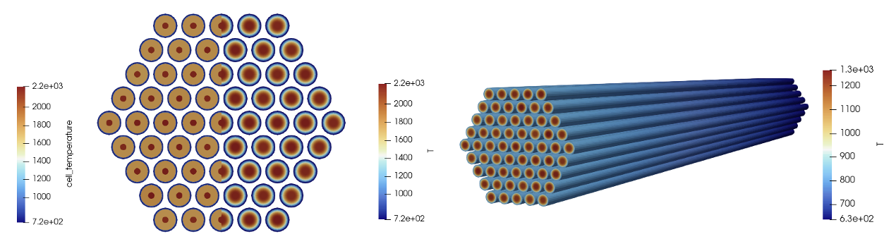
Figure 10: Temperature solution fields for the two-way coupled simulation
Step 3: Three-Way Multiphysics Coupling
For our last simulation, we couple all three solvers - OpenMC, MOOSE heat conduction, and MOOSE subchannel. To describe this model, we will only describe what is now different from the two-way coupling described previously.
Heat Conduction Model
The heat conduction model is the same as that for the two-way coupling, except we remove the function we applied for the cladding surface temperature (it will now be passed into the conduction.i file from the subchannel application). We can also delete the viz.i multiapp which was used just to display data, because we will map the subchannel solution onto the mesh in the openmc.i file, where it will be straightforward to visualize the subchannel solution. The entire file is below.
!include ../common.i

[Mesh]
  [file]
    type = FileMeshGenerator
    file = ../meshes/mesh_in.e
  []
  [delete_coolant]
    type = BlockDeletionGenerator
    input = file
    block = 'sodium'
  []
[]

[Variables]
  [T]
  []
[]

[Kernels]
  [heat_conduction]
    type = HeatConduction
    variable = T
  []
  [heat_source_fuel]
    type = CoupledForce
    variable = T
    v = heat_source
    block = 'fuel'
  []
[]

[Materials]
   [k_helium]
    type = GenericConstantMaterial
    prop_names = 'thermal_conductivity'
    prop_values = '1.5'
    block = 'helium'
  []
   [k_fuel]
    type = GenericConstantMaterial
    prop_names = 'thermal_conductivity'
    prop_values = '2.0'
    block = 'fuel'
  []
   [k_clad]
    type = GenericConstantMaterial
    prop_names = 'thermal_conductivity'
    prop_values = '10.0'
    block = 'clad'
  []
[]

[AuxVariables]
  [T_wall]
    initial_condition = ${inlet_temperature}
  []
  [heat_source]
    # OpenMC computes the variable as constant monomial, so we can receive the
    # field into exactly the same type here (not required, but this will be clearer to
    # visualize in paraview)
    family = MONOMIAL
    order = CONSTANT
    initial_condition = 1e8
    block = 'fuel'
  []
  [q_prime]
    family = MONOMIAL
    order = CONSTANT
    initial_condition = 0.0
    block = 'fuel'
  []
[]

[BCs]
  [cladding_outer_bc]
    type = MatchedValueBC
    variable = T
    v = T_wall
    boundary = '7'
  []
[]

[Executioner]
  type = Transient
[]

[AuxKernels]
  [q_prime]
    type = SpatialUserObjectAux
    variable = q_prime
    user_object = q_prime_uo
    block = 'fuel'
  []
[]

[UserObjects]
  [q_prime_uo]
    type = NearestPointLayeredIntegral
    variable = heat_source
    block = 'fuel'
    direction = z
    points_file = '../pin_centers.txt'
    num_layers = ${n_layers}
    execute_on = 'initial timestep_begin'
  []
[]

[Postprocessors]
  [conduction_power_integral]
    type = ElementIntegralVariablePostprocessor
    variable = heat_source
    block = 'fuel'
    execute_on = 'transfer'
  []
[]

[Outputs]
  exodus = true
[]
Subchannel Model
The subchannel model is the same as that for the single-physics model developed earlier. The linear heat rate will be passed into the subchannel.i file by the heat conduction solver. The entire file is below.
!include ../common.i

# compute the inlet mass flux required to get a bulk temperature rise of 160 K,
# for the imposed power of ${power}. We evaluate the specific heat at the average
# of the inlet and outlet temperatures using a correlation.
temperature = ${fparse 0.5 * (outlet_temperature + inlet_temperature)}
dt = ${fparse 2503.3 - temperature}
Cp = ${fparse 7.3898e5 / dt / dt + 3.154e5 / dt + 1.1340e3 + -2.2153e-1 * dt + 1.1156e-4 * dt * dt}
total_mdot = ${fparse power / Cp / (outlet_temperature - inlet_temperature)}

# compute the mass flux by dividing the mass flowrate by the flow area
flow_area = ${fparse sqrt(3)/2 * (duct_inner_flat_to_flat*1e-2)^2 - 61*pi*(outer_clad_diameter*1e-2)^2/4}

mass_flux_in = ${fparse total_mdot / flow_area}

[TriSubChannelMesh]
  [subchannel]
    type = SCMTriAssemblyMeshGenerator
    nrings = 5
    n_cells = 100
    flat_to_flat = ${fparse duct_inner_flat_to_flat * 1e-2}
    heated_length = ${fparse height * 1e-2}
    pin_diameter = ${fparse outer_clad_diameter * 1e-2}
    pitch = ${fparse pin_pitch * 1e-2}
    dwire = ${fparse wire_diameter * 1e-2}
    hwire = ${fparse wire_pitch * 1e-2}
  []
[]

[ICs]
  [T_IC]
    type = ConstantIC
    variable = T
    value = 500
  []
  [Dpin_IC]
    type = ConstantIC
    variable = Dpin
    value = ${fparse 1e-2 * outer_clad_diameter}
  []
  [q_prime_IC]
    type = ConstantIC
    variable = q_prime
    value = ${fparse power/61/(height*1e-2)}
  []
  [Viscosity_ic]
    type = ViscosityIC
    variable = mu
    p = ${P_out}
    T = T
    fp = sodium
  []
  [rho_ic]
    type = RhoFromPressureTemperatureIC
    variable = rho
    p = ${P_out}
    T = T
    fp = sodium
  []
  [h_ic]
    type = SpecificEnthalpyFromPressureTemperatureIC
    variable = h
    p = ${P_out}
    T = T
    fp = sodium
  []
[]

[FluidProperties]
  [sodium]
    type = PBSodiumFluidProperties
  []
[]

[SubChannel]
  type = TriSubChannel1PhaseProblem
  fp = sodium
  n_blocks = 1
  P_out = ${P_out}
  compute_density = true
  compute_viscosity = true
  compute_power = true
  implicit = true
  segregated = false
  friction_closure = 'cheng_friction'
  mixing_closure = 'cheng_mixing'
  pin_HTC_closure = 'Dittus-Boelter'
  staggered_pressure = false
  P_tol = 1.0e-5
  T_tol = 1.0e-5
[]

[SCMClosures]
  [cheng_friction]
    type = SCMFrictionUpdatedChengTodreas
  []
  [cheng_mixing]
    type = SCMMixingChengTodreas
  []
  [Dittus-Boelter]
    type = SCMHTCDittusBoelter
  []
[]

[AuxKernels]
  [T_in_bc]
    type = ConstantAux
    variable = T
    boundary = inlet
    value = ${inlet_temperature}
    execute_on = 'timestep_begin'
  []
  [mdot_in_bc]
    type = SCMMassFlowRateAux
    variable = mdot
    boundary = inlet
    area = S
    mass_flux = ${mass_flux_in}
    execute_on = 'timestep_begin'
  []
[]

[Postprocessors]
  [power]
    type = SCMPinPowerPostprocessor
  []
  [inlet_temp]
    type = SCMPlanarMean
    variable = T
    height = 0.0
  []
  [outlet_temp]
    type = SCMPlanarMean
    variable = T
    height = ${fparse height * 1e-2}
  []
[]

[Executioner]
  type = Steady
[]

[Outputs]
  exodus = true
[]
OpenMC Model
The OpenMC model is the main application which controls the multiphysics solution. We add a FullSolveMultiApp for the subchannel solver, which will run an entire subchannel simulation each time the subchannel solver is executed. Then, we add four additional transfers, to pass (i) from the conduction solve to the subchannel solver, (ii-iii) retrieve the fluid density and temperature from the subchannel solver, and (iv) pass the clad surface temperature to the conduction model. The entire file is below.
!include ../common.i

[Mesh]
  [file]
    type = FileMeshGenerator
    file = ../meshes/mesh_in.e
  []
[]

[Problem]
  type = OpenMCCellAverageProblem
  power = ${power}
  lowest_cell_level = 2
  scaling = 100
  temperature_blocks = 'helium fuel clad sodium'
  density_blocks = 'sodium'
  xml_directory = '../openmc'

  [Tallies]
    [power]
      type = CellTally
      score = 'kappa_fission'
    []
  []
[]

[ICs]
  [temp]
    type = ConstantIC
    variable = temp
    value = ${inlet_temperature}
  []
  [density]
    type = ConstantIC
    variable = density
    value = ${fparse 1.00423e3 + -0.21390*inlet_temperature+-1.1046e-5*inlet_temperature^2}
  []
[]

[AuxVariables]
  [cell_temperature]
    family = MONOMIAL
    order = CONSTANT
  []
  [cell_density]
    family = MONOMIAL
    order = CONSTANT
  []
[]

[AuxKernels]
  [cell_temperature]
    type = CellTemperatureAux
    variable = cell_temperature
  []
  [cell_density]
    type = CellDensityAux
    variable = cell_density
  []
[]

[Executioner]
  type = Transient
  num_steps = 5
[]

[Outputs]
  exodus = true
[]

[MultiApps]
  [conduction]
    type = TransientMultiApp
    input_files = 'conduction.i'
    sub_cycling = true
    execute_on = timestep_end
  []
  [subchannel]
    type = FullSolveMultiApp
    input_files = 'subchannel.i'
    max_procs_per_app = 1
    execute_on = timestep_begin
  []
[]

[Transfers]
  [power_to_conduction]
    type = MultiAppGeneralFieldNearestLocationTransfer
    to_multi_app = conduction
    source_variable = kappa_fission
    variable = heat_source
    from_postprocessors_to_be_preserved = openmc_power_integral
    to_postprocessors_to_be_preserved = conduction_power_integral
  []
  [solid_temperature_from_conduction]
    type = MultiAppGeneralFieldNearestLocationTransfer
    from_multi_app = conduction
    source_variable = T
    variable = temp
    to_blocks = 'fuel clad helium'
  []

  [linear_heat_rate_to_subchannel]
    type = MultiAppGeneralFieldNearestLocationTransfer
    variable = q_prime
    source_variable = q_prime
    from_multi_app = conduction
    to_multi_app = subchannel
    greedy_search = true
    use_bounding_boxes = false
    to_blocks = 'fuel_pins'
  []
  [fluid_temperature_from_subchannel]
    type = MultiAppGeneralFieldNearestLocationTransfer
    source_variable = T
    variable = temp
    from_multi_app = subchannel
    greedy_search = true
    use_bounding_boxes = false
    to_blocks = 'sodium'
    from_blocks = 'subchannel'
  []
  [fluid_density_from_subchannel]
    type = MultiAppGeneralFieldNearestLocationTransfer
    source_variable = rho
    variable = density
    from_multi_app = subchannel
    greedy_search = true
    use_bounding_boxes = false
    to_blocks = 'sodium'
    from_blocks = 'subchannel'
  []
  [clad_surface_temperature_to_conduction]
    type = MultiAppGeneralFieldNearestLocationTransfer
    from_multi_app = subchannel
    to_multi_app = conduction
    source_variable = Tpin
    variable = T_wall
  []
[]

[Postprocessors]
  [openmc_power_integral]
    type = ElementIntegralVariablePostprocessor
    variable = kappa_fission
    execute_on = 'transfer timestep_end'
  []
[]
Running
To run the three-physics model using 2 MPI ranks and 4 threads per rank (just an example),
mpiexec -np 2 cardinal-opt -i openmc.i --n-threads=4
This will create three output files; openmc_out.e contains the variables from the openmc.i file, openmc_out_conduction0.e contains the variables from the conduction.i file, and openmc_out_subchannel0.e contains the variables from the subchannel.i file.
Figure 11 shows the subchannel fluid temperature solution (left) and the cell temperatures applied to the OpenMC model (right). Note how you can see the typical subchannel discretization from the subchannel solver, but that because the OpenMC cells are pin-centered representations in a hexagonal lattice, the volume-averaged temperatures taken from the subchannel solver are applied to the cells. Note that the cell temperatures in OpenMC, as shown in the image below, do not necessarily look identical to the OpenMC cells because we're only seeing the "shadow" or projection of the OpenMC cell temperatures onto a mesh, whose elements may not conform to the OpenMC cell boundaries.

Figure 11: Temperature computed by the subchannel solver (left) as compared to the cell temperatures applied in OpenMC (right)
The power distribution in the lateral direction is relatively flat, but shows an cosine-like shape in the axial direction due to the leakage on the top and bottom of the assembly. This power distribution is applied to the heat conduction model, resulting in a similar temperature distribution in the fuel (though not identical, as the pin surface temperature follows a typical "s-curve" in the vertical direction as the coolant heats up).

Figure 12: Power computed by OpenMC (top) and the fuel temperature distribution computed by MOOSE (bottom)
You can try several modifications to these files to improve the resolution of the feedback:
Subdivide the model into additional axial layers
Subdivide the OpenMC cells in the fuel into radial rings, to capture radial temperature variations within the fuel pins
Try a MeshTally for the fuel heating, or use a different score such as
heating_localto also compute heat deposited in non-fuel regions