Turbulent Flow in a Pipe
In this tutorial, you will learn how to:
Understand important considerations for running CFD cases
Generate a periodic flow and heat transfer case with NekRS
Compute
Run a Large Eddy Simulation (LES) and perform time averaging
To access this tutorial,
cd cardinal/tutorials/turbulence
Geometry and Computational Model
The domain consists of a pipe flow. The simulation will be set up in non-dimensional units. The diameter of the pipe is 1 and the length is 10. Several different Reynolds numbers will be simulated by varying the fluid viscosity. The sideset numbering in the fluid domain is:
1: side walls
2: inlet
3: outlet
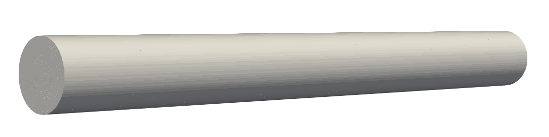
Figure 1: NekRS flow domain. The inlet is located at 0 and the outlet is at 10.
A computational mesh is built using MOOSE's mesh generators, shown below. To generate this mesh, run
cardinal-opt -i pipe.i --mesh-only
mv pipe_in.e pipe.exo
R = 0.5
nl = 8

[Mesh<<<{"href": "../syntax/Mesh/index.html"}>>>]
  [pin]
    type = PolygonConcentricCircleMeshGenerator<<<{"description": "This PolygonConcentricCircleMeshGenerator object is designed to mesh a polygon geometry with optional rings centered inside.", "href": "../source/meshgenerators/PolygonConcentricCircleMeshGenerator.html"}>>>
    num_sides<<<{"description": "Number of sides of the polygon."}>>> = 4
    num_sectors_per_side<<<{"description": "Number of azimuthal sectors per polygon side (rotating counterclockwise from top right face)."}>>> = '8 8 8 8'
    ring_radii<<<{"description": "Radii of major concentric circles (rings)."}>>> = '${fparse 0.5 * R} ${fparse 0.8 * R} ${R}'
    ring_radial_biases<<<{"description": "Values used to create biasing in radial meshing for ring regions."}>>> = '1 1 0.8'
    ring_intervals<<<{"description": "Number of radial mesh intervals within each major concentric circle excluding their boundary layers."}>>> = '1 3 ${nl}'
    ring_block_ids<<<{"description": "Optional customized block ids for each ring geometry block."}>>> = '2 2 2'
    polygon_size<<<{"description": "Size of the polygon to be generated (given as either apothem or radius depending on polygon_size_style)."}>>> = ${fparse 2 * R}
    background_block_ids<<<{"description": "Optional customized block id for the background block."}>>> = '1'
    quad_center_elements<<<{"description": "Whether the center elements are quad or triangular."}>>> = true
    uniform_mesh_on_sides<<<{"description": "Whether the side elements are reorganized to have a uniform size."}>>> = true
    quad_element_type<<<{"description": "Type of the quadrilateral elements to be generated."}>>> = QUAD9
  []
  [delete_background]
    type = BlockDeletionGenerator<<<{"description": "Mesh generator which removes elements from the specified subdomains", "href": "../source/meshgenerators/BlockDeletionGenerator.html"}>>>
    input<<<{"description": "The mesh we want to modify"}>>> = pin
    block<<<{"description": "The list of blocks to be processed (deleted or kept)"}>>> = '1'
  []
  [extrude]
    type = AdvancedExtruderGenerator<<<{"description": "Extrudes a 1D mesh into 2D, or a 2D mesh into 3D, and supports a variable height for each elevation, variable number of layers within each elevation, variable growth factors of axial element sizes within each elevation and remap subdomain_ids, boundary_ids and element extra integers within each elevation as well as interface boundaries between neighboring elevation layers, as well as following a 1D curve and modifying the radial (normal to the extrusion axis) extent of the geometry.", "href": "../source/meshgenerators/AdvancedExtruderGenerator.html"}>>>
    input<<<{"description": "The mesh to extrude"}>>> = delete_background
    direction<<<{"description": "A vector that points in the direction to extrude (note, this will be normalized internally - so don't worry about it here)"}>>> = '0 0 1'
    num_layers<<<{"description": "The number of layers for each elevation - must be num_elevations in length!"}>>> = 40
    heights<<<{"description": "The height of each elevation"}>>> = '10'
  []
  [delete_sides]
    type = BoundaryDeletionGenerator<<<{"description": "Mesh generator which removes side sets", "href": "../source/meshgenerators/BoundaryDeletionGenerator.html"}>>>
    input<<<{"description": "The mesh we want to modify"}>>> = extrude
    boundary_names<<<{"description": "The boundaries to be deleted / kept"}>>> = '1 3'
  []
  [rename]
    type = RenameBoundaryGenerator<<<{"description": "Changes the boundary IDs and/or boundary names for a given set of boundaries defined by either boundary ID or boundary name. The changes are independent of ordering. The merging of boundaries is supported.", "href": "../source/meshgenerators/RenameBoundaryGenerator.html"}>>>
    input<<<{"description": "The mesh we want to modify"}>>> = delete_sides
    old_boundary<<<{"description": "Elements with these boundary ID(s)/name(s) will be given the new boundary information specified in 'new_boundary'"}>>> = '5 6 7'
    new_boundary<<<{"description": "The new boundary ID(s)/name(s) to be given by the boundary elements defined in 'old_boundary'."}>>> = '1 2 3'
  []
  [hex20]
    type = NekMeshGenerator<<<{"description": "Converts MOOSE meshes to element types needed for Nek (Quad8 or Hex20), while optionally preserving curved edges (which were faceted) in the original mesh.", "href": "../source/meshgenerators/NekMeshGenerator.html"}>>>
    input<<<{"description": "The mesh we want to modify"}>>> = rename
  []
[]Inlet-Outlet Conditions
This tutorial will progress through a series of stages of increasing complexity, first beginning with an inlet-outlet boundary condition. The case files are included in the inlet_outlet directory. We initially run this case for a Reynolds number of 100. The initial conditions on velocity will be uniform axial velocity of 1 and for temperature will be a uniform temperature of 0.
[OCCA]
  backend = CPU

[GENERAL]
  polynomialOrder = 3
  numSteps = 10000
  dt = targetCFL=0.5 + initial=1e-4
  writeInterval = 1000

[PRESSURE]
  residualTol = 1e-06

[VELOCITY]
  boundaryTypeMap = W, v, o
  residualTol = 1e-07
  density = 1.0
  viscosity = -100

[TEMPERATURE]
  boundaryTypeMap = f, t, o
  residualTol = 1e-07
  rhoCp = 1.0
  conductivity = -100
#include "udf.hpp"

void UDF_LoadKernels(occa::properties & kernelInfo)
{
}

void UDF_Setup(nrs_t *nrs)
{
  auto mesh = nrs->meshV;

  int n_gll_points = mesh->Np * mesh->Nelements;
  for (int n = 0; n < n_gll_points; ++n)
  {
    nrs->U[n + 0 * nrs->fieldOffset] = 0.0; // x-velocity
    nrs->U[n + 1 * nrs->fieldOffset] = 0.0; // y-velocity
    nrs->U[n + 2 * nrs->fieldOffset] = 1.0; // z-velocity

    nrs->P[n] = 0.0; // pressure

    nrs->cds->S[n + 0 * nrs->fieldOffset] = 0.0; // temperarture
  }
}
void velocityDirichletConditions(bcData *bc)
{
  bc->u = 0.0; // x-velocity
  bc->v = 0.0; // y-velocity
  bc->w = 1.0; // z-velocity
}

void scalarDirichletConditions(bcData *bc)
{
  bc->s = 0.0; // temperature
}

void scalarNeumannConditions(bcData * bc)
{
  bc->flux = 1.0; // heat flux
}
Along the pipe wall, we impose a constant heat flux in non-dimensional units of 1.0. When we non-dimensionalize the energy equation, we divide each term through by the coefficient on the advective term (), which results in a non-dimensional volumetric heat source of
is the temperature difference chosen to scale the dimensional temperature, i.e.
(1)
Therefore, the reference heat flux to obtain the non-dimensional heat flux is simply (taking the scaling for the volumetric heat and multiplying by a length scale to obtain the correct units). This means that the non-dimensional heat flux is scaled as
If we apply a non-dimensional heat flux of 1.0, this means that the dimensional heat flux is
(2)
The total energy deposited in the fluid, via this boundary heat flux, is simply the area integral of the imposed heat flux. From bulk conservation of energy, we know that this energy entering the pipe is equal to .
(3)
where is the surface area through which the heat enters and is the cross-sectional area of the pipe. Inserting Eq. (2) into Eq. Eq. (3) and then rearranging, we find the temperature rise (in dimensional units).
For scaling temperature, we have not yet specified what and are in Eq. (1). Ultimately, these scales do not matter, you can choose any scale! But, it is customary to choose and . With those choices, we can rewrite the right-hand side of the equation above to be in terms of non-dimensional quantities,
Therefore, we expect that in non-dimensional units, our outlet bulk temperature will be if our non-dimensional inlet temperature is 0.
Now that we understand what the various non-dimensional quantities represent for energy, we are ready to run this case. To generate the .re2 mesh, we need to run exo2nek, which will request information via console input. For this example, there are no periodic boundaries or solid portions of the mesh.
exo2nek
To run the case with 12 MPI ranks (just as an example),
nrsmpi fluid 12
Because we output one file every 200 steps, we will obtain 10 output files. To view these files, open the fluid.nek5000 file in a visualization tool such as Paraview or Visit.
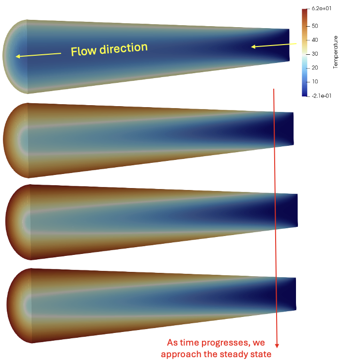
Figure 2: Time evolution of the fluid temperature
From Paraview, we can also extract solution data along lines; for instance, below shows the fluid pressure along the pipe axis. Our mesh is a bit too coarse at the inlet, so there's some bumpiness there in pressure and velocity. The fully-developed pressure gradient, taken by computing the difference in pressure between two points near the outlet,
is around -0.3198 (nondimensional).
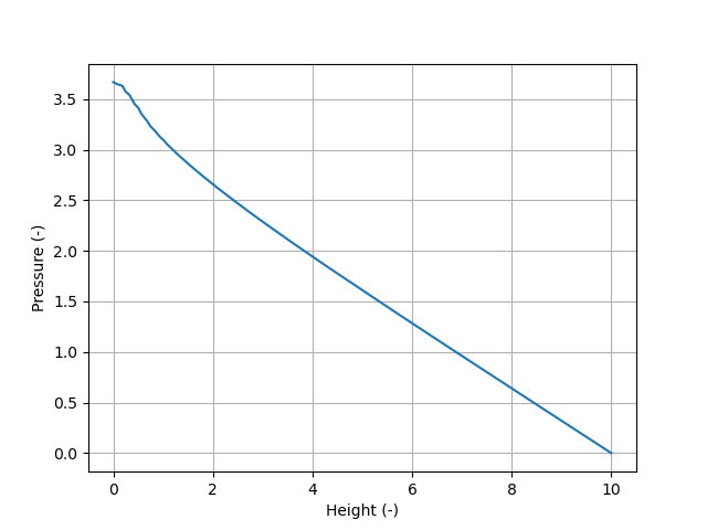
Figure 3: Fluid pressure plotted down the center of the pipe
Monitoring Steady State
Because all our boundary conditions are steady, our flow will reach a steady-state (for laminar flows) or a steady-in-the-mean state (for turbulent flows). We would refer to either of these states as stationarity.'' Generally, you should expect to need several convective units of time to have passed to reach this condition (though this will depend on the details of the flow and on what field you are monitoring). A convective unit is the amount of time required for the flow to move from the inlet to the outlet of the domain one time.
For our domain, we have a length of 10 and a velocity of 1 (both in non-dimensional units), so that a convective unit is 10 non-dimensional time units. Therefore, we need to run for a few of these convective units so that the fluid can "flush out" our initial condition.
The number of convective units you need to reach stationarity depends on the problem and you should remember to inspect all solution fields of interest. Depending on the fluid properties and the initial conditions you chose, temperature could take longer to reach stationarity than velocity, and vice versa.
Steady Flows
For laminar flows or for Reynolds Averaged Navier-Stokes (RANS) with steady boundary conditions, we expect to reach an actual steady state in the solution fields. For these cases, you can inspect the field files to get a sense of when this stationarity has been reached, and you can also add C++ code to the .udf file to print out various solution scalar quantities (e.g. maximum/minimum values, norms along lines, etc.).
Another easy way to monitor steady state is using Cardinal. For example, the input below will run your NekRS case and automatically terminate once the relative change in your solution between two successive time steps and is less than a provided tolerance . This check is performed for all auxiliary variables individually in your problem, if you are using check_aux = True.
The solution is the auxiliary system solution, meaning one long vector containing all of the auxiliary variables (which you need to explicitly pass from NekRS's internals into MOOSE variables using FieldTransfers. The norm above is scaled by so that if you have a very small time step, the solution wouldn't change very much in such a short window of time (even if the steady state has not been reached yet). You can also inspect postprocessors to see how they vary during the simulation, for instance the bulk outlet temperature (which should be above the inlet bulk temperature (in non-dimensional terms) once reaching the steady state.
[Mesh<<<{"href": "../syntax/Mesh/index.html"}>>>]
  type = NekRSMesh
  volume = true
[]

[Problem<<<{"href": "../syntax/Problem/index.html"}>>>]
  type = NekRSProblem
  casename<<<{"description": "Case name for the NekRS input files; this is <case> in <case>.par, <case>.udf, <case>.oudf, and <case>.re2."}>>> = pipe

  [FieldTransfers<<<{"href": "../syntax/Problem/FieldTransfers/index.html"}>>>]
    [temp]
      type = NekFieldVariable<<<{"description": "Reads/writes volumetric field data between NekRS and MOOSE."}>>>
      direction<<<{"description": "Direction in which to send data"}>>> = from_nek
      field<<<{"description": "NekRS field variable to read/write; defaults to the name of the object"}>>> = temperature
    []
    [vel_z]
      type = NekFieldVariable<<<{"description": "Reads/writes volumetric field data between NekRS and MOOSE."}>>>
      direction<<<{"description": "Direction in which to send data"}>>> = from_nek
      field<<<{"description": "NekRS field variable to read/write; defaults to the name of the object"}>>> = velocity_z
    []
  []
[]

[Executioner<<<{"href": "../syntax/Executioner/index.html"}>>>]
  type = Transient
  steady_state_detection = true
  steady_state_tolerance = 1e-3
  check_aux = true

  [TimeStepper<<<{"href": "../syntax/Executioner/TimeStepper/index.html"}>>>]
    type = NekTimeStepper
  []
[]

[Postprocessors<<<{"href": "../syntax/Postprocessors/index.html"}>>>]
  # this quantity will be 40 if we run to the steady-state
  [outlet_bulk_T]
    type = NekMassFluxWeightedSideAverage<<<{"description": "Mass flux weighted average of a field over a boundary in the NekRS mesh", "href": "../source/postprocessors/NekMassFluxWeightedSideAverage.html"}>>>
    field<<<{"description": "Field to apply this object to"}>>> = temperature
    boundary<<<{"description": "Boundary ID(s) for which to compute the postprocessor"}>>> = '3'
  []
[]Turbulent Flows
For turbulent flow modeling using LES or Direct Numerical Simulation (DNS), the flow will reach statistical stationarity. Methods to evaluate this will be described later in this tutorial.
Periodic Boundary Conditions
For many flows of interest, we are only interested in the fully-developed solution. We can use inlet-outlet conditions for these scenarios, provided our domain is sufficiently long enough and we only use the solution towards the outlet (once reaching fully-developed conditions). However, this can result in a very long flow domain. For instance, turbulent flow in a round pipe requires a development length of around
which can be 20-30 pipe diameters. For laminar flow, because the turbulent transport is not aiding in the lateral transport across the pipe, the development length can be even higher (on the order of 100 pipe diameters at the upper range of the laminar regime). Therefore, if our interest is only in the fully-developed state, a natural choice would be to instead model the pipe with periodic boundary conditions.
The case files for this periodic case are in the periodic subdirectory.
Setting up a Periodic Mesh
To establish a periodic mesh, our 3-D fluid mesh must have two faces which are periodic (identical topology). The element IDs on those faces must be shifted by an equal shift. For instance, if one mesh face has three elements with IDs 1, 2, 3 then the corresponding paired periodic mesh face would need to have IDs 9, 10, 11 (an equal shift of 8 for each). You can easily attain this by generating a 2-D mesh of your geometry, and then extruding it. This is how we made the exodus mesh for our pipe. However, we cannot simply use the pipe.re2 we generated for the inlet-outlet case earlier. We need to re-run exo2nek and inform NekRS that we have one periodic pair of boundaries, and that those boundary IDs are 2 and 3.
exo2nek
Now, we have a new pipe.re2 file. For periodic cases, we need to have a .usr file to (i) set the boundary IDs of any sidesets which are to be periodic, to zero and (ii) renormalize any remaining boundary IDs so that they are sequential beginning at 1.
c-----------------------------------------------------------------------
      subroutine useric(i,j,k,eg)
      include 'SIZE'
      include 'TOTAL'
      include 'NEKUSE'
      integer i,j,k,e,eg

      return
      end
c-----------------------------------------------------------------------
      subroutine userchk
      include 'SIZE'
      include 'TOTAL'

      return
      end
c-----------------------------------------------------------------------
      subroutine usrdat
      include 'SIZE'
      include 'TOTAL'

      return
      end
c-----------------------------------------------------------------------
      subroutine usrdat2()
      include 'SIZE'
      include 'TOTAL'

      do iel=1,nelt
      do ifc=1,2*ndim
         if (boundaryID(ifc,iel).eq. 1) then
           boundaryID(ifc,iel) = 1
         else if (boundaryID(ifc,iel).eq. 2) then
           boundaryID(ifc,iel) = 0
         else if (boundaryID(ifc,iel) .eq. 3) then
           boundaryID(ifc,iel) = 0
         endif
      enddo
      enddo

      return
      end
c-----------------------------------------------------------------------
      subroutine usrdat3
      include 'SIZE'
      include 'TOTAL'

      return
      end
c-----------------------------------------------------------------------
Then, in our .par file, we will only refer to the non-periodic boundaries which remain (so, our boundaryTypeMap fields will only list the boundary condition for the solid walls since that is the only boundary remaining in our mesh).
[OCCA]
  backend = CPU

[GENERAL]
  polynomialOrder = 3
  numSteps = 10000
  dt = targetCFL=0.5 + initial=1e-4
  writeInterval = 100
  constFlowRate = meanVelocity=1.0 + direction=Z

[PRESSURE]
  residualTol = 1e-06

[VELOCITY]
  boundaryTypeMap = W
  residualTol = 1e-07
  density = 1.0
  viscosity = -100

[TEMPERATURE]
  boundaryTypeMap = f
  residualTol = 1e-07
  rhoCp = 1.0
  conductivity = -100
Note that in our .oudf file, we also only need to prescribe boundary conditions for the non-periodic boundaries.
void scalarNeumannConditions(bcData * bc)
{
  bc->flux = 1.0; // heat flux
}

@kernel void periodicSource(const dlong Nelements, const dlong offset, const dfloat gamma, @restrict const dfloat * vel_z, @restrict dfloat * QVOL)
{
  for(dlong e=0;e<Nelements;++e;@outer(0)){
    for(int n=0;n<p_Np;++n;@inner(0)){
      const int id = e*p_Np + n;
      QVOL[id] = - 1.0 * vel_z[id + 2 * offset] * gamma;
    }
  }
}
Periodic Flow and Temperature
NekRS treats the Gauss-Lobatto-Legendre (GLL) points and their corresponding degrees-of-freedom (DOFs) no different than interior nodes. That is, the velocity, pressure, temperature, etc. at the nodes on one periodic face are identical to those on the corresponding periodic face.
For the inlet/outlet case, the pressure gradient becomes constant in the fully-developed region. Similarly, for a constant heat flux, the temperature gradient also becomes constant. Physically, this means that for the fully-developed flow that the pressure and temperature will have a constant streamwise gradient - so by definition, it's not possible for the pressure field to be identical on the inlet and outlet face (and neither for temperature). Therefore, what NekRS actually solves for in periodic flow cases is a decomposed pressure and a decomposed temperature .
With a constant heat flux, we know that the temperature at a height will just be shifted by some amount relative to the temperature at height 0.
(4)
From energy conservation, is
(5)
For this example, our heat flux is 1.0, and our nondimensional density, velocity, and specific heat are also 1.0. Therefore, .
Now, we want to recast the energy equation in a way such that the outlet temperature does indeed equal the inlet temperature (so that our periodic boundary conditions work). Inserting the above into the conservation of energy equation,
(6)
In this way, by adding a heat sink term , the actual quantity we are solving for with the energy equation is the periodic temperature field . This field can be a function of height if the geometry itself varies with , such as in wire-wrapped pin bundles (e.g. see Dutra et al. (2024)). In other words, the representation in Eq. (4) does allow the periodic temperature field to vary in (i.e. if you were to plot along a vertical line, you would not see a constant temperature) unless your geometry had no change in the cross-sectional geometry with height (like is the case for our simple pipe).
We need to add this heat sink, , to our problem ourselves. This will require adding a kernel to the energy equation. Our resulting temperature field that we compute will represent the fully-developed temperature, but scaled so that its average is zero. Although including this heat sink is all that is strictly necessary, it is a good idea to also explicitly subtract out any numerical drift in the temperature average. Over long integration times, even if the bulk average is still a small number (e.g. ), this can slowly drift over time.
#include "udf.hpp"

static occa::kernel periodicSourceKernel;

void UDF_LoadKernels(occa::properties & kernelInfo)
{
  periodicSourceKernel = oudfBuildKernel(kernelInfo, "periodicSource");
}

void userq(nrs_t * nrs, double time, occa::memory o_S, occa::memory o_FS)
{
  auto mesh = nrs->cds->mesh[0];
  dfloat R = 0.5;
  dfloat q_dagger = 1.0;
  periodicSourceKernel(mesh->Nelements, nrs->fieldOffset, 2 / R * q_dagger, nrs->o_U, o_FS);

  // prevent any numerical drift by subtracting out the volume-average temperature
  const dfloat Tbar =
    platform->linAlg->innerProd(mesh->Nlocal, o_S, mesh->o_LMM, platform->comm.mpiComm) / mesh->volume;
  platform->linAlg->add(mesh->Nlocal, -Tbar, o_S);
}

void UDF_Setup(nrs_t *nrs)
{
  auto mesh = nrs->meshV;

  int n_gll_points = mesh->Np * mesh->Nelements;
  for (int n = 0; n < n_gll_points; ++n)
  {
    nrs->U[n + 0 * nrs->fieldOffset] = 0.0; // x-velocity
    nrs->U[n + 1 * nrs->fieldOffset] = 0.0; // y-velocity
    nrs->U[n + 2 * nrs->fieldOffset] = 1.0; // z-velocity

    nrs->P[n] = 0.0; // pressure

    nrs->cds->S[n + 0 * nrs->fieldOffset] = 0.0; // temperature
  }

  udf.sEqnSource = &userq;
}
void scalarNeumannConditions(bcData * bc)
{
  bc->flux = 1.0; // heat flux
}

@kernel void periodicSource(const dlong Nelements, const dlong offset, const dfloat gamma, @restrict const dfloat * vel_z, @restrict dfloat * QVOL)
{
  for(dlong e=0;e<Nelements;++e;@outer(0)){
    for(int n=0;n<p_Np;++n;@inner(0)){
      const int id = e*p_Np + n;
      QVOL[id] = - 1.0 * vel_z[id + 2 * offset] * gamma;
    }
  }
}
Likewise for pressure, NekRS will solve for the pressure field superimposed on top of the constant-pressure-gradient arising from fully-developed flow.
(7)
To correctly set up the flow aspects of a periodic case, all we need to add is the following line to the .par file, where the meanVelocity should be the mean velocity (for our non-dimensional case, this is the mean value of which is just 1 because we choose a reference velocity scale to be the mean dimensional axial velocity). The direction indicates which coordinate direction represents the periodic direction.
constFlowRate = meanVelocity=1.0 + direction=Z
For the round pipe, our pressure distribution we will solve for with NekRS is simply zero (because our true pressure distribution is simply a constant axial gradient). Whereas in Eq. (5) we know how to scale back from our non-dimensional fully-developed temperature, you don't need to manually make any changes to kernels/etc. to accomplish the periodic flow (aside from setting the constFlowRate). When running the case, NekRS will print to the screen the fully developed pressure gradient () in Eq. Eq. (7) as the scale term. For instance, for the time step shown below, the fully developed pressure gradient is 3.0882e-1 (compare this to the value we estimated from our inlet/outlet case earlier).
Time Step 623, time = 11.0732, dt = 0.016456
copying solution to nek
S00      : iter 011  resNorm0 4.63e-07  resNorm 8.63e-08
projP    : resNorm0 1.56e-07  resNorm 9.08e-12  ratio = 1.721e+04  5/8
P        : iter 001  resNorm0 9.08e-12  resNorm 1.46e-12
UVW      : iter 035  resNorm0 2.21e-03  resNorm 7.00e-08  divErrNorms 3.23e-14 3.00e-07
flowRate : uBulk0 9.97e-01  uBulk 1.00e+00  err 2.22e-16  scale 3.08822e-01
step= 623  t= 1.10731611e+01  dt=1.6e-02  C= 0.48  elapsedStep= 5.07e-02s  elapsedStepSum= 3.55035e+01s
We are now ready to run this case. We will use the Cardinal input from the inlet/outlet case earlier to easily monitor steady state detection. To run with 12 ranks (just an example),
mpiexec -np 12 cardinal-opt -i nek.i
You will notice that with the periodic case, we reach a steady-state much faster than the inlet/outlet case. Pressure is effectively zero. Shown below is the temperature, .
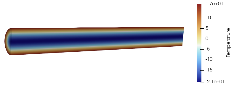
Figure 4: NekRS temperature solution for periodic boundary conditions.
Turbulent Simulations with NekRS
Directly solving the Navier-Stokes equations, without any additional coupled equations (RANS) or without any filters to drain energy from the shortest wavelengths (ac), is called DNS. The highest fidelity methods require more runtime, and hence there is a tradeoff in fidelity and computing requirements. In this section and those that follow, we will simulate our pipe at a Reynolds number of 5000, well within the turbulent regime.
RANS, LES, and DNS
<! add general intro to RANS, LES, DNS >
In many cases, RANS simulations are performed alongside LES and/or DNS in order to help guide mesh resolution requirements.
<! image of interplay>
<! ### Mesh Resolution Requirements>
Computing
In Cardinal, you can compute the maximum, minimum, or average value of on a given sideset in NekRS using the NekYPlus postprocessor. For wall-resolved simulations (without the use of wall functions), it is recommended to have a mesh refined near the wall with . NekRS does not currently have wall functions.
is a non-dimensional length scale that is uniquely defined at each node on the wall as
where is the distance from the wall to the nearest GLL point, is the kinematic viscosity ( for non-dimensional simulations), and is the friction velocity. is defined as
where is the wall shear stress and is the density (1.0 for non-dimensional simulations). The wall shear stress is the magnitude of the viscous force vector on the wall, considering only the components of that vector which act tangential to the wall. In tensor notation, the -th component of the viscous force is . Therefore, to subtract off any contributions along the direction (perpendicular to the surface), we write
where is the -the component of the viscous force vector, which when dotted with the unit normal () is the component of the viscous force vector perpendicular to the surface. To subtract out this perpendicular component, we multiply by to correctly subtract out the -th component of the perpendicular component from the -th component of the viscous force vector .
When generating a mesh, it can be helpful to estimate (in addition to monitoring it with NekYPlus during the simulation). To obtain a rough estimate of , note that it can be related to the Darcy friction factor as
giving
where for non-dimensional solutions. It is common to simply take the Blasius correlation for flow along a flat plate, since this is just an approximation anyways and you can rely on the computed during the run to obtain final guidance on mesh resolution near the wall.
So, for the scenario in this tutorial, we could open an output file and obtain the coordinates at a point on the boundary to compute (use the red dot with a question mark on the toolbar and then hover over a node). From the two nodes shown below, we'd estimate to be around 0.000365.
Figure 5: NekRS mesh (showing the GLL points) and with the Paraview hover feature
Then, we would estimate for a flat plate for (definitely not a pipe, so we are just crudely estimating ). This would give an approximate on the wall as 0.38 in this mesh. We can compare this value with the NekYPlus postprocessor, and find we did a pretty good job! The maximum on the mesh, after one convective unit, is around 0.5.
Underresolved Turbulence
If your mesh is not fine enough, the typical observation will be that your velocity attains high, unphysical oscillations in value and/or a very high Courant-Friedrichs-Lewy (CFL) number (which in NekRS could cause the solve to abort).
<! example image>
Tripping a Simulation to Turbulence
For simple geometries, it may be necessary to add some 3-D behavior to your initial condition for velocity in order for the simulation to trip into turbulence. For example, below shows the velocity distribution for as solved by NekRS when the initial condition is a parabola in the -direction. No turbulence develops even after running this simulation for 20 convective units.
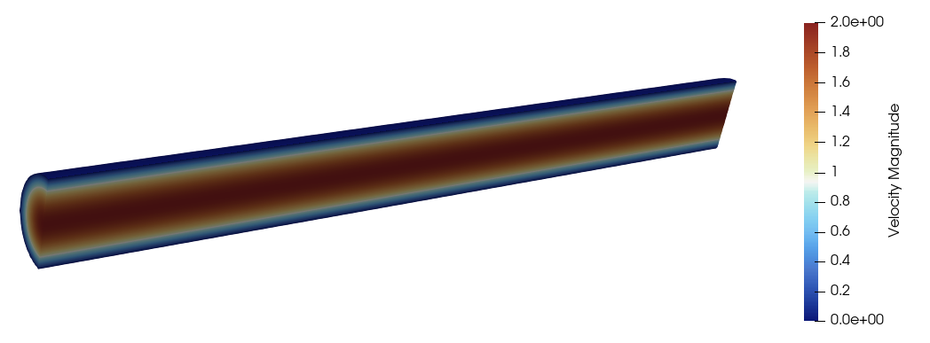
Figure 6: NekRS velocity solution after running for 20 convective units at Reynolds number of 5000
We can set the initial condition to have some perturbation in the and components of velocity, such as
This will trip the simulation into turbulence. For instance, a few snapshots at different convective units are shown below.
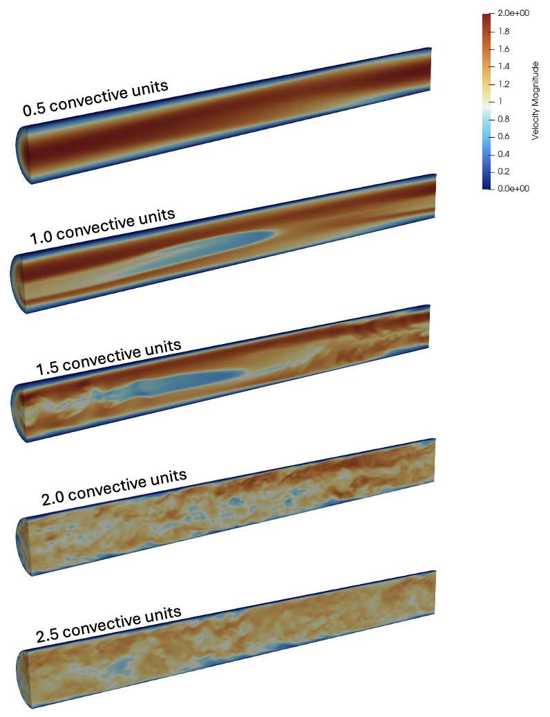
Figure 7: NekRS velocity solution after running a few convective units at Reynolds number of 5000
Large Eddy Simulation
In this section, we will model flow in a pipe at a Reynolds number of 5000 using LES. These input files are in the tutorials/turbulence/les directory. LES in NekRS uses a filter to drain energy from the shortest wavelengths (highest frequencies) of the velocity, temperature, and scalar(s) solutions. For a description on the theoretical background, see this page. Here, we focus on the practical aspects of running LES with NekRS.
To run an LES simulation with NekRS, simply enable the filtering in the .par file with the filtering, filterWeight, and filterModes options. Generally recommended settings, for polynomial order greater than or equal to 5, are shown in the file below. The LES filtering in NekRS is spectrally convergent, so you can always choose a filter setting and then conduct a p-refinement study to ensure an adequately converged solution.
[OCCA]
  backend = CPU

[GENERAL]
  polynomialOrder = 7
  numSteps = 100000
  dt = targetCFL=0.5 + initial=1e-4
  writeInterval = 2000
  constFlowRate = meanVelocity=1.0 + direction=Z

  # comment out to run DNS (no LES filtering)
  filtering = hpfrt
  filterWeight = 5.0
  filterModes = 2

[PRESSURE]
  residualTol = 1e-06

[VELOCITY]
  boundaryTypeMap = W
  residualTol = 1e-07
  density = 1.0
  viscosity = -5000

[TEMPERATURE]
  boundaryTypeMap = f
  residualTol = 1e-07
  rhoCp = 1.0
  conductivity = -5000
The other input files are largely unchanged, but we will add time averaging operations in the .udf file, discussed next.
Time-Averaging
LES and DNS both compute time-dependent flow fields. For comparison with RANS and some experimental measurements, it is helpful to time-average the flow fields to find the mean flow. Recall from the Reynolds decomposition that an instantaneous quantity can be decomposed into a mean and a fluctuation (with zero mean but nonzero variance). For instance, for the -th component of velocity, this is
The time average is defined as
NekRS provides functionality to time-average its instantaneous velocity/pressure/temperature solutions during the run. This section of the tutorial is an abridged version of the time-averaging documentation on the NekRS website.
In the .udf file, we simply add a few lines to register the time-averaging kernel in UDF_LoadKernels and UDF_Setup. Then in UDF_ExecuteStep we call the time-averaging operation at the same frequency as we write output files (this is not required, but common).
#include "udf.hpp"
#include "plugins/tavg.hpp"

static occa::kernel periodicSourceKernel;

void UDF_LoadKernels(occa::properties & kernelInfo)
{
  periodicSourceKernel = oudfBuildKernel(kernelInfo, "periodicSource");
  tavg::buildKernel(kernelInfo);
}

void userq(nrs_t * nrs, double time, occa::memory o_S, occa::memory o_FS)
{
  auto mesh = nrs->cds->mesh[0];
  dfloat R = 0.5;
  dfloat q_dagger = 1.0;
  periodicSourceKernel(mesh->Nelements, nrs->fieldOffset, 2 / R * q_dagger, nrs->o_U, o_FS);

  // prevent any numerical drift by subtracting out the volume-average temperature
  const dfloat Tbar =
    platform->linAlg->innerProd(mesh->Nlocal, o_S, mesh->o_LMM, platform->comm.mpiComm) / mesh->volume;
  platform->linAlg->add(mesh->Nlocal, -Tbar, o_S);
}

void UDF_Setup(nrs_t *nrs)
{
  auto mesh = nrs->meshV;

  std::string name;
  setupAide &options = platform->options;
  options.getArgs("RESTART FILE NAME", name);

  // only set initial conditions if there is no restart file
  if (name == "")
  {
    int n_gll_points = mesh->Np * mesh->Nelements;
    for (int n = 0; n < n_gll_points; ++n)
    {
      // comment out to see flow if no initial perturbation is applied to the x, y velocity components
      nrs->U[n + 0 * nrs->fieldOffset] = 0.2 * std::cos(mesh->z[n]); // x-velocity
      nrs->U[n + 1 * nrs->fieldOffset] = 0.2 * std::sin(mesh->z[n]); // y-velocity

      dfloat r = std::sqrt(mesh->x[n] * mesh->x[n] + mesh->y[n] * mesh->y[n]) * 2.0;
      nrs->U[n + 2 * nrs->fieldOffset] = -2 * (r * r - 1); // z-velocity

      nrs->P[n] = 0.0; // pressure

      nrs->cds->S[n + 0 * nrs->fieldOffset] = 0.0; // temperature
    }
  }

  // this will call userchk in the fortran file, which does the time averaging
  nek::userchk();

  tavg::setup(nrs);
  udf.sEqnSource = &userq;
}

void UDF_ExecuteStep(nrs_t * nrs, double time, int tstep)
{
  tavg::run(time);

  if (nrs->isOutputStep)
    tavg::outfld();
}
When running NekRS, this will now create three additional output files on each output step. Since our casename is pipe, these will be named
avgpipe0.f*: these contain the time-averaged fields (first-order moments), i.e. , , , etc. By default, the window for time averaging resets each time the averaging routine is called. In other words, if an output file is written on time steps 1000, 1500, and 3000, thenavgpipe0.f00001contains the time average of the solution fields over time steps 0-1000;avgpipe0.f00002contains the time average of the solution fields over time steps 1000-1500; andavgpipe0.f00003contains the time average of the solution fields over time steps 1500-3000.rmspipe0.f*: averages of the squares (second-order moments) e.g. , , and for temperature, .rm2pipe0.f*: averages of the mixed correlations , , .
The mean Reynolds stress tensor has components which can then be computed as
and so on for the other components.
To time-average together the averages, you will put in the userchk() routine in the .usr file a call to a function which will average together the various avgpipe0.f* files. This function takes as input the index of the file from which you want to begin the cumulative average, and the index of the file from which you want to end the cumulative average. For instance, if you want to average together files avgpipe0.f00035, avgpipe0.f00036, and avgpipe0.f00037, call the function as call average_files("pipe", 35, 37).
      subroutine average_files(inbase,startf,stopf)
      implicit none
      include 'SIZE'
      include 'TOTAL'
      include 'AVG'

      character*(*) inbase
      character*8   ftail
      integer lbase,startf,stopf,n,n2,i,j
      logical ifxyo_s

      n=nx1*ny1*nz1*nelv
      n2=nx2*ny2*nz2*nelv

      atime=0.0
      call rzero(uavg,n)
      call rzero(vavg,n)
      call rzero(wavg,n)
      call rzero(pavg,n2)
      do j=1,ldimt
        call rzero(tavg(1,1,1,1,j),n)
      enddo
      do i=startf,stopf
        if(i.lt.10) then
          write(ftail,'(a7,i1)')'0.f0000',i
        elseif(i.lt.100) then
          write(ftail,'(a6,i2)')'0.f000',i
        elseif(i.lt.1000) then
          write(ftail,'(a5,i3)')'0.f00',i
        endif
        call blank(initc(1),132)
        initc(1)=trim(inbase)//ftail

        call restart(1)

        atime=atime+time
        call add2s2(uavg,vx,time,n)
        call add2s2(vavg,vy,time,n)
        call add2s2(wavg,vz,time,n)
        call add2s2(pavg,pr,time,n2)
        do j=1,ldimt
          call add2s2(tavg(1,1,1,1,j),t(1,1,1,1,j),time,n)
        enddo
      enddo
      time=atime
      call cmult(uavg,1.0/atime,n)
      call cmult(vavg,1.0/atime,n)
      call cmult(wavg,1.0/atime,n)
      call cmult(pavg,1.0/atime,n2)
      do j=1,ldimt
        call cmult(tavg(1,1,1,1,j),1.0/atime,n)
      enddo

      call copy (vx,uavg,n)
      call copy (vy,vavg,n)
      call copy (vz,wavg,n)
      call copy (pr,pavg,n2)
      do j=1,ldimt
        call copy(t(1,1,1,1,j),tavg(1,1,1,1,j),n)
      enddo

      ifxyo_s = ifxyo
      ifxyo=.true.

      call prepost (.true.,'tav')

      ifxyo = ifxyo_s

      return
      end

c-----------------------------------------------------------------------
      subroutine useric(i,j,k,eg)
      include 'SIZE'
      include 'TOTAL'
      include 'NEKUSE'

      return
      end
c-----------------------------------------------------------------------
      subroutine userchk
      include 'SIZE'
      include 'TOTAL'

c change this to 1 to do the averaging. Before you can set this to 1,
c you need to have run your case. 35 is the file to start reading, 50
c is the file to stop reading. 'pipe' is the casename
      ifaveraging=0
      if (ifaveraging.eq.1) then
       call average_files("pipe",35, 50)
       call exitt()
      endif

      return
      end
c-----------------------------------------------------------------------
      subroutine usrdat
      include 'SIZE'
      include 'TOTAL'

      return
      end
c-----------------------------------------------------------------------
      subroutine usrdat2()
      include 'SIZE'
      include 'TOTAL'

      do iel=1,nelt
      do ifc=1,2*ndim
         if (boundaryID(ifc,iel).eq. 1) then
           boundaryID(ifc,iel) = 1
           cbc(ifc,iel,1)= 'W  '
         else if (boundaryID(ifc,iel).eq. 2) then
           boundaryID(ifc,iel) = 0
         else if (boundaryID(ifc,iel) .eq. 3) then
           boundaryID(ifc,iel) = 0
         endif
      enddo
      enddo

      return
      end
c-----------------------------------------------------------------------
      subroutine usrdat3
      include 'SIZE'
      include 'TOTAL'

      common /scrach_o1/ w1(lx1*ly1*lz1*lelv),
     $                   w2(lx1*ly1*lz1*lelv),
     $                   w3(lx1*ly1*lz1*lelv),
     $                   w4(lx1*ly1*lz1*lelv),
     $                   w5(lx1*ly1*lz1*lelv)

      common /scrach_o2/ ywd(lx1,ly1,lz1,lelv)

      COMMON /NRSSCPTR/ nrs_scptr(1)
      integer*8         nrs_scptr

      call distf(ywd,1,'W  ',w1,w2,w3,w4,w5)

      nrs_scptr(1) = loc(ywd)

      return
      end
c-----------------------------------------------------------------------
To call this userchk function, put a call to nek::userchk() in the UDF_Setup routine. Then, you will run your simulation in two stages:
Run your case as normal, with
ifaveraging=0. This will generate all the nominal output files.Run the case a second time, but change
ifaveraging=0toifaveraging=1. Theexitt()call will terminate right after the time-average-of-time-averages is formed and not run any time steps. This will create a new file, withtavas a prefix. This file will contain the cumulative time average for the window specified.
Several (sometimes many) convective units will be required to reach a statistically stationary state. Common choices could be 10-100 convective units to wait before you begin the cumulative average. Another 10-100 convective units would then be required after this point to obtain a long enough cumulative average so that the average itself becomes steady.
Viewing the Individual Time-Averaged Slices
When generating the time-averaged files, the default behavior is for the time to reset in each file once the new time averaging window begins. Paraview will not be able to open these avg, rms, and rm2 files as-is because they may not have a monotonically increasing simulation time. To convert the files into a form which can be read by Paraview, run from the folder where the output files are located,
python ../../../../scripts/change_time.py --case pipe
where ../../../../scripts/change_time.py is the path to the chang_time.py script in the cardinal/scripts directory.
To undo this action, pass the --reset flag to the change_time.py script. The times must be unmodified to be able to time average the averaged files together.
python ../../../../scripts/change_time.py --case pipe --reset
References
- C. Bourdot Dutra, L. Aldeia Macahdo, and E. Merzari.
Direct numerical simulation of heat transfer in a 7-pin wire-wrapped rod bundle.
Nuclear Science and Engineering, 198:1439–1454, 2024.
doi:10.1080/00295639.2023.2246778.[Export]