Volume Junction

A general conservation law equation can be expressed as

\pdat+f=0\eqc\pd{a}{t} + \nabla\cdot\mathbf{f} = 0 \eqc

where aa is the conserved quantity. Integrating this equation over a volume Ω\Omega gives

Ω\pdatdΩ+ΩfdΩ=0\eqp\int\limits_{\Omega} \pd{a}{t} d\Omega + \int\limits_{\Omega} \nabla\cdot\mathbf{f} d\Omega = 0 \eqp

The time derivative can be expressed as follows:

Ω\pdatdΩ=\ddtaˉV\eqc\int\limits_{\Omega} \pd{a}{t} d\Omega = \ddt{\bar{a} V} \eqc

where aˉ\bar{a} is the average of aa over Ω\Omega:

aˉ1VΩadΩ\eqc\bar{a} \equiv \frac{1}{V}\int\limits_{\Omega} a d\Omega \eqc

and VΩdΩV \equiv \int\limits_{\Omega} d\Omega.

The flux term can be expressed as follows:

ΩfdΩ=ΓfndΓ\eqc\int\limits_{\Omega} \nabla\cdot\mathbf{f} d\Omega = \int\limits_\Gamma \mathbf{f}\cdot\mathbf{n} d\Gamma \eqc

where Γ\Gamma is the surface of Ω\Omega, and n\mathbf{n} is the outward normal vector at a position on the surface.

Now consider that Γ\Gamma is partitioned into a number of regions: Γ=ΓwallΓflow\Gamma = \Gamma_{\text{wall}} \cup \Gamma_{\text{flow}}, where Γflow=i=1NΓflow,i\Gamma_{\text{flow}} = \bigcup\limits_{i=1}^{N} \Gamma_{\text{flow},i}. The surface Γwall\Gamma_{\text{wall}} corresponds to a wall, and the surface Γflow,i\Gamma_{\text{flow},i} corresponds to a flow surface, across which a fluid may pass. The number of flow surfaces on the volume is denoted by NN. See Figure Figure 1 for an illustration.

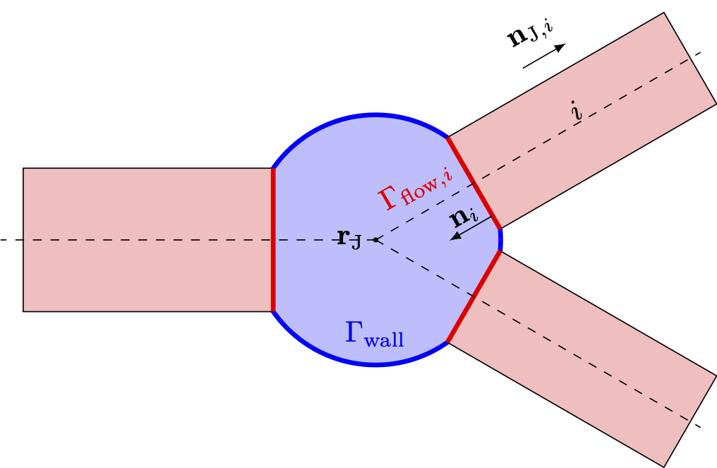
Figure 1: Volume junction illustration.

Now the surface integral can be expressed as follows:

ΓfndΓ=ΓwallfndΓ+i=1NΓflow,ifndΓ\eqp\int\limits_\Gamma \mathbf{f}\cdot\mathbf{n} d\Gamma = \int\limits_{\Gamma_{\text{wall}}} \mathbf{f}\cdot\mathbf{n} d\Gamma + \sum\limits_{i=1}^N \int\limits_{\Gamma_{\text{flow},i}} \mathbf{f}\cdot\mathbf{n} d\Gamma \eqp

Now consider that the flux f\mathbf{f} is constant over each flow surface, and that each flow surface is flat (thus making n\mathbf{n} constant over the surface). Then,

Γflow,ifndΓ=finJ,iAi\eqc\int\limits_{\Gamma_{\text{flow},i}} \mathbf{f}\cdot\mathbf{n} d\Gamma = \mathbf{f}_i \cdot \mathbf{n}_{J,i} A_i \eqc

where nJ,i=ni\mathbf{n}_{J,i} = -\mathbf{n}_i, and ni\mathbf{n}_i is the outward-facing (from the channel perspective) normal of channel ii at the interface with the junction.

Now the wall surface integral term needs to be discussed. At this point, we consider the particular conservation laws of interest. Starting with conservation of mass, where a=ρa = \rho and f=fmassρu\mathbf{f} = \mathbf{f}^{\text{mass}} \equiv \rho \mathbf{u}:

ΓwallfndΓ=ΓwallρundΓ=0\eqc\int\limits_{\Gamma_{\text{wall}}} \mathbf{f}\cdot\mathbf{n} d\Gamma = \int\limits_{\Gamma_{\text{wall}}} \rho \mathbf{u}\cdot\mathbf{n} d\Gamma = 0 \eqc

owing to the wall boundary condition un=0\mathbf{u}\cdot\mathbf{n} = 0.

For conservation of momentum in the xx-direction, a=ρua = \rho u and f=fmom,xρuu+pex\mathbf{f} = \mathbf{f}^{\text{mom},x} \equiv \rho u \mathbf{u} + p \mathbf{e}_x:

ΓwallfndΓ=Γwall\prρuu+pexndΓ=ΓwallpnxdΓ\eqp\int\limits_{\Gamma_{\text{wall}}} \mathbf{f}\cdot\mathbf{n} d\Gamma = \int\limits_{\Gamma_{\text{wall}}} \pr{\rho u \mathbf{u} + p \mathbf{e}_x}\cdot\mathbf{n} d\Gamma = \int\limits_{\Gamma_{\text{wall}}} p n_x d\Gamma \eqp

Then, assuming the pressure to be constant along the surface, equal to the average pressure in the volume,

ΓwallpnxdΓ=pˉΓwallnxdΓ\eqp\int\limits_{\Gamma_{\text{wall}}} p n_x d\Gamma = \bar{p}\int\limits_{\Gamma_{\text{wall}}} n_x d\Gamma \eqp

Using the Gauss divergence theorem,

ΓndΓ=0\eqc\int\limits_{\Gamma} \mathbf{n} d\Gamma = \mathbf{0} \eqcΓwallndΓ+i=1NnJ,iAi=0\eqc\int\limits_{\Gamma_{\text{wall}}} \mathbf{n} d\Gamma + \sum\limits_{i=1}^N \mathbf{n}_{J,i} A_i = \mathbf{0} \eqcΓwallndΓ=i=1NnJ,iAi\eqp\int\limits_{\Gamma_{\text{wall}}} \mathbf{n} d\Gamma = - \sum\limits_{i=1}^N \mathbf{n}_{J,i} A_i \eqp

Therefore,

pˉΓwallnxdΓ=pˉi=1Nni,xAi\eqp\bar{p} \int\limits_{\Gamma_{\text{wall}}} n_x d\Gamma = \bar{p} \sum\limits_{i=1}^N n_{i,x} A_i \eqp

Conservation of momentum in the yy and zz directions proceeds similarly.

Finally, conservation of energy has a=ρEa = \rho E and f=fenergy\prρE+pu\mathbf{f} = \mathbf{f}^{\text{energy}} \equiv \pr{\rho E + p}\mathbf{u}:

ΓwallfndΓ=Γwall\prρE+pundΓ=0\eqc\int\limits_{\Gamma_{\text{wall}}} \mathbf{f}\cdot\mathbf{n} d\Gamma = \int\limits_{\Gamma_{\text{wall}}} \pr{\rho E + p}\mathbf{u}\cdot\mathbf{n} d\Gamma = 0 \eqc

again owing to wall boundary conditions.

Putting everything together and denoting the volume-average quantities with the subscript JJ gives

\ddt\prρVJ=i=1NfimassnJ,iAi\eqc\ddt{\pr{\rho V}_J} = -\sum\limits_{i=1}^N \mathbf{f}^{\text{mass}}_i \cdot \mathbf{n}_{J,i} A_i \eqc\ddt\prρuVJ=i=1Nfimom,xnJ,iAipJi=1Nni,xAi\eqc\ddt{\pr{\rho u V}_J} = -\sum\limits_{i=1}^N \mathbf{f}^{\text{mom},x}_i \cdot \mathbf{n}_{J,i} A_i - p_J \sum\limits_{i=1}^N n_{i,x} A_i \eqc\ddt\prρvVJ=i=1Nfimom,ynJ,iAipJi=1Nni,yAi\eqc\ddt{\pr{\rho v V}_J} = -\sum\limits_{i=1}^N \mathbf{f}^{\text{mom},y}_i \cdot \mathbf{n}_{J,i} A_i - p_J \sum\limits_{i=1}^N n_{i,y} A_i \eqc\ddt\prρwVJ=i=1Nfimom,znJ,iAipJi=1Nni,zAi\eqc\ddt{\pr{\rho w V}_J} = -\sum\limits_{i=1}^N \mathbf{f}^{\text{mom},z}_i \cdot \mathbf{n}_{J,i} A_i - p_J \sum\limits_{i=1}^N n_{i,z} A_i \eqc\ddt\prρEVJ=i=1NfienergynJ,iAi\eqp\ddt{\pr{\rho E V}_J} = -\sum\limits_{i=1}^N \mathbf{f}^{\text{energy}}_i \cdot \mathbf{n}_{J,i} A_i \eqp

The fluxes are computed using a numerical flux function,

F(UL,UR,nL,R,t1,t2)=[fnmassfnmom,nfnmom,t1fnmom,t2fnenergy]\eqc\mathcal{F}(\mathbf{U}_\text{L}, \mathbf{U}_\text{R}, \mathbf{n}_{\text{L},\text{R}}, \mathbf{t}_1, \mathbf{t}_2) = \left[\begin{array}{c} f^\text{mass}_n \\ f^{\text{mom},n}_n \\ f^{\text{mom},t_1}_n \\ f^{\text{mom},t_2}_n \\ f^\text{energy}_n \end{array}\right] \eqc

where the vector nL,R\mathbf{n}_{\text{L},\text{R}} is the outward unit vector from the "L" state to the "R" state, and t1\mathbf{t}_1 and t2\mathbf{t}_2 are arbitrary unit vectors forming an orthonormal basis with nL,R\mathbf{n}_{\text{L},\text{R}}.

The "L" state is taken to be the junction, and the "R" state is taken to be the channel ii:

UJ,i[ρJρJuJρJEJ]\eqc\mathbf{U}_{\text{J},i} \equiv \left[\begin{array}{c} \rho_\text{J} \\ \rho_\text{J} \mathbf{u}_\text{J} \\ \rho_\text{J} E_\text{J} \end{array}\right] \eqcUi[ρiρiui,ddiρiEi]\eqc\mathbf{U}_i \equiv \left[\begin{array}{c} \rho_i \\ \rho_i u_{i,d} \mathbf{d}_i \\ \rho_i E_i \end{array}\right] \eqcnL,RnJ,i\eqc\mathbf{n}_{\text{L},\text{R}} \equiv \mathbf{n}_{\text{J},i} \eqc[fn,imassfn,imom,nfn,imom,t1fn,imom,t2fn,ienergy]=F(UJ,i,Ui,nJ,i,t1,i,t2,i)\eqc\left[\begin{array}{c} f^\text{mass}_{n,i} \\ f^{\text{mom},n}_{n,i} \\ f^{\text{mom},t_1}_{n,i} \\ f^{\text{mom},t_2}_{n,i} \\ f^\text{energy}_{n,i} \end{array}\right] = \mathcal{F}(\mathbf{U}_{\text{J},i}, \mathbf{U}_i, \mathbf{n}_{\text{J},i}, \mathbf{t}_{1,i}, \mathbf{t}_{2,i}) \eqc

where di\mathbf{d}_i is the local orientation vector for flow channel ii, equal or opposite to ni\mathbf{n}_i, and ui,du_{i,d} is the component of the channel ii velocity in the direction di\mathbf{d}_i.

The input velocities here are in the global Cartesian basis {ex,ey,ez}\{\mathbf{e}_x, \mathbf{e}_y, \mathbf{e}_z\}, whereas the numerical flux function returns momentum components in the normal basis {nL,R,t1,t2}\{\mathbf{n}_{\text{L},\text{R}}, \mathbf{t}_1, \mathbf{t}_2\}, so one must perform a change of basis afterward:

fn,imom,x=(fn,imom,nnJ,i+fn,imom,t1t1,i+fn,imom,t2t2,i)ex\eqpf^{\text{mom},x}_{n,i} = (f^{\text{mom},n}_{n,i} \mathbf{n}_{\text{J},i} + f^{\text{mom},t_1}_{n,i} \mathbf{t}_{1,i} + f^{\text{mom},t_2}_{n,i} \mathbf{t}_{2,i}) \cdot \mathbf{e}_x \eqpfn,imom,y=(fn,imom,nnJ,i+fn,imom,t1t1,i+fn,imom,t2t2,i)ey\eqpf^{\text{mom},y}_{n,i} = (f^{\text{mom},n}_{n,i} \mathbf{n}_{\text{J},i} + f^{\text{mom},t_1}_{n,i} \mathbf{t}_{1,i} + f^{\text{mom},t_2}_{n,i} \mathbf{t}_{2,i}) \cdot \mathbf{e}_y \eqpfn,imom,z=(fn,imom,nnJ,i+fn,imom,t1t1,i+fn,imom,t2t2,i)ez\eqpf^{\text{mom},z}_{n,i} = (f^{\text{mom},n}_{n,i} \mathbf{n}_{\text{J},i} + f^{\text{mom},t_1}_{n,i} \mathbf{t}_{1,i} + f^{\text{mom},t_2}_{n,i} \mathbf{t}_{2,i}) \cdot \mathbf{e}_z \eqp

However, as shown by Hong and Kim (2011) and noted in Daude and Galon (2018), the choice of junction state given above leads to spurious pressure jumps at the junction, so the normal component of the velocity in the junction state UJ,i\mathbf{U}_{\text{J},i} is modified as follows:

u~J,i=u~J,i,nnJ,i+uJ,i,t1t1,i+uJ,i,t2t2,i\eqc\tilde{\mathbf{u}}_{\text{J},i} = \tilde{u}_{\text{J},i,n} \mathbf{n}_{\text{J},i} + u_{\text{J},i,t_1} \mathbf{t}_{1,i} + u_{\text{J},i,t_2} \mathbf{t}_{2,i} \eqcu~J,i,n=ui,nGi(ui,nuJ,i,n)\eqc\tilde{u}_{\text{J},i,n} = u_{i,n} - \mathcal{G}_i \left(u_{i,n} - u_{\text{J},i,n}\right) \eqc

with ui,nui,ddinJ,iu_{i,n} \equiv u_{i,d} \mathbf{d}_i \cdot \mathbf{n}_{\text{J},i} and uJ,i,nuJnJ,iu_{\text{J},i,n} \equiv \mathbf{u}_\text{J} \cdot \mathbf{n}_{\text{J},i} and

Gi=12(1sgn(ui,n))min(ui,nuJ,i,ncJ,i,1)\eqc\mathcal{G}_i = \frac{1}{2} \left(1 - \text{sgn}(u_{i,n})\right) \min\left(\frac{\left|u_{i,n} - u_{\text{J},i,n}\right|}{c_{\text{J},i}}, 1\right) \eqc

with cJ,imax(ci,cJ)c_{\text{J},i} \equiv \max(c_i, c_\text{J}), where cc is sound speed.

References

  1. F. Daude and P. Galon. A finite-volume approach for compressible single- and two-phase flows in flexible pipelines with fluid-structure interaction. Journal of Computational Physics, 362:375–408, 2018. URL: https://www.sciencedirect.com/science/article/pii/S0021999118301207, doi:https://doi.org/10.1016/j.jcp.2018.01.055.[BibTeX]
  2. Seok Hong and Chongam Kim. A new finite volume method on junction coupling and boundary treatment for flow network system analyses. International Journal for Numerical Methods in Fluids, 65:707 – 742, 02 2011. doi:10.1002/fld.2212.[BibTeX]