POD Reduced Basis Surrogate
This example is meant to demonstrate how a POD reduced basis surrogate model is trained and used on a parametric problem.
Problem statement
The full-order model is a one energy group, fixed-source diffusion-reaction problem, adopted from Prince and Ragusa (2019). The geometry for this problem is presented in Figure 1. The problem has four different material regions, from which three (1, 2 and 3) act as fixed sources.
).](../../../large_media/stochastic_tools/surrogates/pod_rb/2d_multiregion_geometry.png)
Figure 1: The geometry of the diffusion-reaction problem used in this example (Prince and Ragusa (2019)).
The fixed-source diffusion-reaction problem with space dependent coefficients can be expressed as:
(1)where is the diffusion coefficient, is the reaction coefficient, is the fixed source term and field variable is the solution of interest. Furthermore, denotes the internal domain, without the boundaries, which can be partitioned into four sub-domains corresponding to the four material regions (, , and ). This equation needs to be supplemented with boundary conditions. For the symmetry lines (dashed lines in Figure 1, denoted by ) a homogeneous Neumann condition is used:
while the rest of the boundaries (in the reflector, denoted by ) are treated with homogeneous Dirichlet conditions:
This problem is parametric in a sense that the solution depends on the values of the coefficients and the source: . In this example, material region-wise constant coefficients and source terms are considered yielding eight uncertain parameters altogether (assuming that Region 4 does not have a source). The material properties in each region have Uniform distributions () specified in Table 1 with and being the lower and upper bounds.
Table 1: The distributions of the uncertain parameters used in this problem (Prince and Ragusa (2019)).
| Parameter | Symbol | Distribution |
|---|---|---|
| Diffusion coefficient in Region 1 | ||
| Diffusion coefficient in Region 2 | ||
| Diffusion coefficient in Region 3 | ||
| Diffusion coefficient in Region 4 | ||
| Reaction coefficient in Region 1 | ||
| Reaction coefficient in Region 2 | ||
| Reaction coefficient in Region 3 | ||
| Reaction coefficient in Region 4 | ||
| Fixed-source in Region 1 | ||
| Fixed-source in Region 2 | ||
| Fixed-source in Region 3 |
It is important to mention that POD-RB surrogates are only efficient when the original problem has an affine decomposition. For more information about affine decomposition see PODReducedBasisTrainer. Luckily, the problem at hand has an affine decomposition in the following form:
where , and take the values of , and when and 0 otherwise.
Solving the problem without uncertain parameters
The first step towards creating a POD-RB surrogate model is the generation of a full-order problem which can solve Eq. (1) with fixed parameters. There are three important factors that need to be considered while preparing the input file for this problem:
The user must specify vector tags in the
Problemblock for each component in the affine decomposition of the system. In this example, as shown in Listing 1, 8 vector tags are specified for the eight uncertain parameters. These do not introduce extra work in the full-order model, however they help to identify the affine components throughout the training phase.Listing 1: Complete input file for the heat equation problem in this study.
(contrib/moose/modules/stochastic_tools/examples/surrogates/pod_rb/2d_multireg/sub.i)[Problem<<<{"href": "../../../syntax/Problem/index.html"}>>>] type = FEProblem extra_tag_vectors = 'diff0 diff1 diff2 diff3 abs0 abs1 abs2 abs3 src0 src1 src2' []The input file has to reflect the affine decomposition of the problem. This means that the
Kernels,BCsandMaterialshave to be created in a way that they correspond to the components in the affine decomposition. This is shown in Listing 2. Note that a separate kernel has been created for every single term in the decomposition. The vector tags in theProblemblock are then applied to these kernels to ensure that the affine components are correctly identified throughout the training phase.Listing 2: Complete input file for the heat equation problem in this study.
(contrib/moose/modules/stochastic_tools/examples/surrogates/pod_rb/2d_multireg/sub.i)[Kernels<<<{"href": "../../../syntax/Kernels/index.html"}>>>] [diff0] type = MatDiffusion<<<{"description": "Diffusion equation Kernel that takes an isotropic Diffusivity from a material property", "href": "../../../source/kernels/MatDiffusion.html"}>>> variable<<<{"description": "The name of the variable that this residual object operates on"}>>> = psi diffusivity<<<{"description": "The diffusivity value or material property"}>>> = D0 extra_vector_tags<<<{"description": "The extra tags for the vectors this Kernel should fill"}>>> = 'diff0' block<<<{"description": "The list of blocks (ids or names) that this object will be applied"}>>> = 0 [] [diff1] type = MatDiffusion<<<{"description": "Diffusion equation Kernel that takes an isotropic Diffusivity from a material property", "href": "../../../source/kernels/MatDiffusion.html"}>>> variable<<<{"description": "The name of the variable that this residual object operates on"}>>> = psi diffusivity<<<{"description": "The diffusivity value or material property"}>>> = D1 extra_vector_tags<<<{"description": "The extra tags for the vectors this Kernel should fill"}>>> = 'diff1' block<<<{"description": "The list of blocks (ids or names) that this object will be applied"}>>> = 1 [] [diff2] type = MatDiffusion<<<{"description": "Diffusion equation Kernel that takes an isotropic Diffusivity from a material property", "href": "../../../source/kernels/MatDiffusion.html"}>>> variable<<<{"description": "The name of the variable that this residual object operates on"}>>> = psi diffusivity<<<{"description": "The diffusivity value or material property"}>>> = D2 extra_vector_tags<<<{"description": "The extra tags for the vectors this Kernel should fill"}>>> = 'diff2' block<<<{"description": "The list of blocks (ids or names) that this object will be applied"}>>> = 2 [] [diff3] type = MatDiffusion<<<{"description": "Diffusion equation Kernel that takes an isotropic Diffusivity from a material property", "href": "../../../source/kernels/MatDiffusion.html"}>>> variable<<<{"description": "The name of the variable that this residual object operates on"}>>> = psi diffusivity<<<{"description": "The diffusivity value or material property"}>>> = D3 extra_vector_tags<<<{"description": "The extra tags for the vectors this Kernel should fill"}>>> = 'diff3' block<<<{"description": "The list of blocks (ids or names) that this object will be applied"}>>> = 3 [] [abs0] type = MaterialReaction variable = psi coefficient = absxs0 extra_vector_tags = 'abs0' block = 0 [] [abs1] type = MaterialReaction variable = psi coefficient = absxs1 extra_vector_tags = 'abs1' block = 1 [] [abs2] type = MaterialReaction variable = psi coefficient = absxs2 extra_vector_tags = 'abs2' block = 2 [] [abs3] type = MaterialReaction variable = psi coefficient = absxs3 extra_vector_tags = 'abs3' block = 3 [] [src0] type = BodyForce<<<{"description": "Demonstrates the multiple ways that scalar values can be introduced into kernels, e.g. (controllable) constants, functions, and postprocessors. Implements the weak form $(\\psi_i, -f)$.", "href": "../../../source/kernels/BodyForce.html"}>>> variable<<<{"description": "The name of the variable that this residual object operates on"}>>> = psi value<<<{"description": "Coefficient to multiply by the body force term"}>>> = 1 extra_vector_tags<<<{"description": "The extra tags for the vectors this Kernel should fill"}>>> = 'src0' block<<<{"description": "The list of blocks (ids or names) that this object will be applied"}>>> = 0 [] [src1] type = BodyForce<<<{"description": "Demonstrates the multiple ways that scalar values can be introduced into kernels, e.g. (controllable) constants, functions, and postprocessors. Implements the weak form $(\\psi_i, -f)$.", "href": "../../../source/kernels/BodyForce.html"}>>> variable<<<{"description": "The name of the variable that this residual object operates on"}>>> = psi value<<<{"description": "Coefficient to multiply by the body force term"}>>> = 1 extra_vector_tags<<<{"description": "The extra tags for the vectors this Kernel should fill"}>>> = 'src1' block<<<{"description": "The list of blocks (ids or names) that this object will be applied"}>>> = 1 [] [src2] type = BodyForce<<<{"description": "Demonstrates the multiple ways that scalar values can be introduced into kernels, e.g. (controllable) constants, functions, and postprocessors. Implements the weak form $(\\psi_i, -f)$.", "href": "../../../source/kernels/BodyForce.html"}>>> variable<<<{"description": "The name of the variable that this residual object operates on"}>>> = psi value<<<{"description": "Coefficient to multiply by the body force term"}>>> = 1 extra_vector_tags<<<{"description": "The extra tags for the vectors this Kernel should fill"}>>> = 'src2' block<<<{"description": "The list of blocks (ids or names) that this object will be applied"}>>> = 2 [] [] [Materials<<<{"href": "../../../syntax/Materials/index.html"}>>>] [D0] type = GenericConstantMaterial<<<{"description": "Declares material properties based on names and values prescribed by input parameters.", "href": "../../../source/materials/GenericConstantMaterial.html"}>>> prop_names<<<{"description": "The names of the properties this material will have"}>>> = D0 prop_values<<<{"description": "The values associated with the named properties"}>>> = 1 block<<<{"description": "The list of blocks (ids or names) that this object will be applied"}>>> = 0 [] [D1] type = GenericConstantMaterial<<<{"description": "Declares material properties based on names and values prescribed by input parameters.", "href": "../../../source/materials/GenericConstantMaterial.html"}>>> prop_names<<<{"description": "The names of the properties this material will have"}>>> = D1 prop_values<<<{"description": "The values associated with the named properties"}>>> = 1 block<<<{"description": "The list of blocks (ids or names) that this object will be applied"}>>> = 1 [] [D2] type = GenericConstantMaterial<<<{"description": "Declares material properties based on names and values prescribed by input parameters.", "href": "../../../source/materials/GenericConstantMaterial.html"}>>> prop_names<<<{"description": "The names of the properties this material will have"}>>> = D2 prop_values<<<{"description": "The values associated with the named properties"}>>> = 1 block<<<{"description": "The list of blocks (ids or names) that this object will be applied"}>>> = 2 [] [D3] type = GenericConstantMaterial<<<{"description": "Declares material properties based on names and values prescribed by input parameters.", "href": "../../../source/materials/GenericConstantMaterial.html"}>>> prop_names<<<{"description": "The names of the properties this material will have"}>>> = D3 prop_values<<<{"description": "The values associated with the named properties"}>>> = 1 block<<<{"description": "The list of blocks (ids or names) that this object will be applied"}>>> = 3 [] [absxs0] type = GenericConstantMaterial<<<{"description": "Declares material properties based on names and values prescribed by input parameters.", "href": "../../../source/materials/GenericConstantMaterial.html"}>>> prop_names<<<{"description": "The names of the properties this material will have"}>>> = absxs0 prop_values<<<{"description": "The values associated with the named properties"}>>> = 1 block<<<{"description": "The list of blocks (ids or names) that this object will be applied"}>>> = 0 [] [absxs1] type = GenericConstantMaterial<<<{"description": "Declares material properties based on names and values prescribed by input parameters.", "href": "../../../source/materials/GenericConstantMaterial.html"}>>> prop_names<<<{"description": "The names of the properties this material will have"}>>> = absxs1 prop_values<<<{"description": "The values associated with the named properties"}>>> = 1 block<<<{"description": "The list of blocks (ids or names) that this object will be applied"}>>> = 1 [] [absxs2] type = GenericConstantMaterial<<<{"description": "Declares material properties based on names and values prescribed by input parameters.", "href": "../../../source/materials/GenericConstantMaterial.html"}>>> prop_names<<<{"description": "The names of the properties this material will have"}>>> = absxs2 prop_values<<<{"description": "The values associated with the named properties"}>>> = 1 block<<<{"description": "The list of blocks (ids or names) that this object will be applied"}>>> = 2 [] [absxs3] type = GenericConstantMaterial<<<{"description": "Declares material properties based on names and values prescribed by input parameters.", "href": "../../../source/materials/GenericConstantMaterial.html"}>>> prop_names<<<{"description": "The names of the properties this material will have"}>>> = absxs3 prop_values<<<{"description": "The values associated with the named properties"}>>> = 1 block<<<{"description": "The list of blocks (ids or names) that this object will be applied"}>>> = 3 [] []The values for each uncertain parameter have to be set to 1 by default. This is necessary because the PODReducedBasisTrainer uses the same input file to create the affine constituent operators. This ensures that the mentioned operators are not influenced by the parameter-dependent multipliers. Of course, these values are not fixed and are changed by the main application throughout the simulations to values aligned with those in Table 1. However, the default values in the input file should be set to one. This is shown in Listing 2 as well.
Training surrogate models
For the details of the training procedure of a POD-RB surrogate, see PODReducedBasisTrainer. The first step is the collection of data, which involves the repeated execution of the full-order problem with different parameter combinations and the saving of the full solution vectors. These solution vectors are often referred to as snapshots and this naming is preferred in this example as well. This step is managed by the main input file which creates parameter samples, transfers them to the sub-application and collects the results from the completed computations.
The snapshot collection phase starts with the definition of the distributions in the Distributions block. The uniform distributions for all the 8 uncertain parameters are specified as:
[Distributions<<<{"href": "../../../syntax/Distributions/index.html"}>>>]
  [D012_dist]
    type = Uniform<<<{"description": "Continuous uniform distribution.", "href": "../../../source/distributions/Uniform.html"}>>>
    lower_bound<<<{"description": "Distribution lower bound"}>>> = 0.2
    upper_bound<<<{"description": "Distribution upper bound"}>>> = 0.8
  []
  [D1_dist]
    type = Uniform<<<{"description": "Continuous uniform distribution.", "href": "../../../source/distributions/Uniform.html"}>>>
    lower_bound<<<{"description": "Distribution lower bound"}>>> = 0.2
    upper_bound<<<{"description": "Distribution upper bound"}>>> = 0.8
  []
  [D2_dist]
    type = Uniform<<<{"description": "Continuous uniform distribution.", "href": "../../../source/distributions/Uniform.html"}>>>
    lower_bound<<<{"description": "Distribution lower bound"}>>> = 0.2
    upper_bound<<<{"description": "Distribution upper bound"}>>> = 0.8
  []
  [D3_dist]
    type = Uniform<<<{"description": "Continuous uniform distribution.", "href": "../../../source/distributions/Uniform.html"}>>>
    lower_bound<<<{"description": "Distribution lower bound"}>>> = 0.15
    upper_bound<<<{"description": "Distribution upper bound"}>>> = 0.6
  []
  [absxs0_dist]
    type = Uniform<<<{"description": "Continuous uniform distribution.", "href": "../../../source/distributions/Uniform.html"}>>>
    lower_bound<<<{"description": "Distribution lower bound"}>>> = 0.0425
    upper_bound<<<{"description": "Distribution upper bound"}>>> = 0.17
  []
  [absxs1_dist]
    type = Uniform<<<{"description": "Continuous uniform distribution.", "href": "../../../source/distributions/Uniform.html"}>>>
    lower_bound<<<{"description": "Distribution lower bound"}>>> = 0.065
    upper_bound<<<{"description": "Distribution upper bound"}>>> = 0.26
  []
  [absxs2_dist]
    type = Uniform<<<{"description": "Continuous uniform distribution.", "href": "../../../source/distributions/Uniform.html"}>>>
    lower_bound<<<{"description": "Distribution lower bound"}>>> = 0.04
    upper_bound<<<{"description": "Distribution upper bound"}>>> = 0.16
  []
  [absxs3_dist]
    type = Uniform<<<{"description": "Continuous uniform distribution.", "href": "../../../source/distributions/Uniform.html"}>>>
    lower_bound<<<{"description": "Distribution lower bound"}>>> = 0.005
    upper_bound<<<{"description": "Distribution upper bound"}>>> = 0.02
  []
  [src_dist]
    type = Uniform<<<{"description": "Continuous uniform distribution.", "href": "../../../source/distributions/Uniform.html"}>>>
    lower_bound<<<{"description": "Distribution lower bound"}>>> = 5
    upper_bound<<<{"description": "Distribution upper bound"}>>> = 20
  []
[]As a next step, the underlying distributions are sampled to create parameter combinations. This is done using a LatinHypercube defined in the Samplers block. It is visible that 100 samples are prepared, meaning that 100 snapshots will be collected for the generation of the surrogates.
[Samplers<<<{"href": "../../../syntax/Samplers/index.html"}>>>]
  [sample]
    type = LatinHypercube<<<{"description": "Latin Hypercube Sampler.", "href": "../../../source/samplers/LatinHypercubeSampler.html"}>>>
    distributions<<<{"description": "The distribution names to be sampled, the number of distributions provided defines the number of columns per matrix."}>>> = 'D012_dist D012_dist D012_dist D3_dist
                     absxs0_dist absxs1_dist absxs2_dist absxs3_dist
                     src_dist src_dist src_dist'
    num_rows<<<{"description": "The size of the square matrix to generate."}>>> = 100
    execute_on<<<{"description": "The list of flag(s) indicating when this object should be executed. For a description of each flag, see https://mooseframework.inl.gov/source/interfaces/SetupInterface.html."}>>> = PRE_MULTIAPP_SETUP
    max_procs_per_row<<<{"description": "This will ensure that the sampler is partitioned properly when 'MultiApp/*/max_procs_per_app' is specified. It is not recommended to use otherwise."}>>> = 1
  []
[]To be able to create the reduced operators for the surrogate model, a custom MultiApp, PODFullSolveMultiApp, has been created. This object is responsible for executing sub-problems using different combinations of parameter values provided by the sampler. The secondary function of this object is to create the action of the full-order operators on the basis functions of the reduced subspace. Therefore, this object has to be executed twice in the same simulation. It is visible that unlike a regular SamplerFullSolveMultiApp, this custom object has to know certain parameters of the trainer as well.
[MultiApps<<<{"href": "../../../syntax/MultiApps/index.html"}>>>]
  [sub]
    type = PODFullSolveMultiApp<<<{"description": "Creates a full-solve type sub-application for each row of a Sampler matrix. On second call, this object creates residuals for a PODReducedBasisTrainer with given basis functions.", "href": "../../../source/multiapps/PODFullSolveMultiApp.html"}>>>
    input_files<<<{"description": "The input file for each App.  If this parameter only contains one input file it will be used for all of the Apps.  When using 'positions_from_file' it is also admissable to provide one input_file per file."}>>> = sub.i
    sampler<<<{"description": "The Sampler object to utilize for creating MultiApps."}>>> = sample
    trainer_name<<<{"description": "Trainer object that contains the solutions for different samples."}>>> = 'pod_rb'
    execute_on<<<{"description": "The list of flag(s) indicating when this object should be executed. For a description of each flag, see https://mooseframework.inl.gov/source/interfaces/SetupInterface.html."}>>> = 'timestep_begin final'
    max_procs_per_app<<<{"description": "Maximum number of processors to give to each App in this MultiApp.  Useful for restricting small solves to just a few procs so they don't get spread out"}>>> = 1
  []
[]In terms of the Transfers block, besides sending the actual parameter samples to the sub-applications, in this intrusive procedure, the snapshots need to be collected from the sub-applications, the basis functions need to be sent back to different sub-applications and the action of the operators on the basis functions need to be collected as well. This requires four transfer objects. The two custom types (PODSamplerSolutionTransfer and PODResidualTransfer) are specifically used to support PODReducedBasisTrainer at this moment.
[Transfers<<<{"href": "../../../syntax/Transfers/index.html"}>>>]
  [param]
    type = SamplerParameterTransfer<<<{"description": "Copies Sampler data to a SamplerReceiver object.", "href": "../../../source/transfers/SamplerParameterTransfer.html"}>>>
    to_multi_app<<<{"description": "The name of the MultiApp to transfer the data to"}>>> = sub
    sampler<<<{"description": "A the Sampler object that Transfer is associated.."}>>> = sample
    parameters<<<{"description": "A list of parameters (on the sub application) to control with the Sampler data. The order of the parameters listed here should match the order of the items in the Sampler."}>>> = 'Materials/D0/prop_values
                  Materials/D1/prop_values
                  Materials/D2/prop_values
                  Materials/D3/prop_values
                  Materials/absxs0/prop_values
                  Materials/absxs1/prop_values
                  Materials/absxs2/prop_values
                  Materials/absxs3/prop_values
                  Kernels/src0/value
                  Kernels/src1/value
                  Kernels/src2/value'
    execute_on<<<{"description": "The list of flag(s) indicating when this object should be executed. For a description of each flag, see https://mooseframework.inl.gov/source/interfaces/SetupInterface.html."}>>> = 'timestep_begin'
    check_multiapp_execute_on<<<{"description": "When false the check between the multiapp and transfer execute on flags is not performed."}>>> = false
  []
  [data]
    type = PODSamplerSolutionTransfer<<<{"description": "Transfers solution vectors from the sub-applications to a a container in the Trainer object and back.", "href": "../../../source/transfers/PODSamplerSolutionTransfer.html"}>>>
    from_multi_app<<<{"description": "The name of the MultiApp to receive data from"}>>> = sub
    sampler<<<{"description": "A the Sampler object that Transfer is associated.."}>>> = sample
    trainer_name<<<{"description": "Trainer object that contains the solutions for different samples."}>>> = 'pod_rb'
    execute_on<<<{"description": "The list of flag(s) indicating when this object should be executed. For a description of each flag, see https://mooseframework.inl.gov/source/interfaces/SetupInterface.html."}>>> = 'timestep_begin'
    check_multiapp_execute_on<<<{"description": "When false the check between the multiapp and transfer execute on flags is not performed."}>>> = false
  []
  [mode]
    type = PODSamplerSolutionTransfer<<<{"description": "Transfers solution vectors from the sub-applications to a a container in the Trainer object and back.", "href": "../../../source/transfers/PODSamplerSolutionTransfer.html"}>>>
    to_multi_app<<<{"description": "The name of the MultiApp to transfer the data to"}>>> = sub
    sampler<<<{"description": "A the Sampler object that Transfer is associated.."}>>> = sample
    trainer_name<<<{"description": "Trainer object that contains the solutions for different samples."}>>> = 'pod_rb'
    execute_on<<<{"description": "The list of flag(s) indicating when this object should be executed. For a description of each flag, see https://mooseframework.inl.gov/source/interfaces/SetupInterface.html."}>>> = 'final'
    check_multiapp_execute_on<<<{"description": "When false the check between the multiapp and transfer execute on flags is not performed."}>>> = false
  []
  [res]
    type = PODResidualTransfer<<<{"description": "Transfers residual vectors from the sub-application to a a container in the Trainer object.", "href": "../../../source/transfers/PODResidualTransfer.html"}>>>
    from_multi_app<<<{"description": "The name of the MultiApp to receive data from"}>>> = sub
    sampler<<<{"description": "A the Sampler object that Transfer is associated.."}>>> = sample
    trainer_name<<<{"description": "Trainer object that contains the solutions for different samples."}>>> = 'pod_rb'
    execute_on<<<{"description": "The list of flag(s) indicating when this object should be executed. For a description of each flag, see https://mooseframework.inl.gov/source/interfaces/SetupInterface.html."}>>> = 'final'
    check_multiapp_execute_on<<<{"description": "When false the check between the multiapp and transfer execute on flags is not performed."}>>> = false
  []
[]Next, the PODReducedBasisTrainer is set up in the Trainers block. The trainer stores the snapshots and uses them to create basis functions for the reduced subspaces. Furthermore, it is also responsible for creating the reduced-order operators, therefore it needs to be executed twice in the training process. The trainer object needs to know what variable needs to be reduced and the names of the vector tags from the sub-application to be able to identify the affine constituent operators. Furthermore, using the "tag_types" input argument, the user has to specify if the reduced affine constituent operator acts on the variable or not. The ordering must be the same as the names of the vector tags. The meaning of the energy retention limits is discussed in PODReducedBasisTrainer.
[Trainers<<<{"href": "../../../syntax/Trainers/index.html"}>>>]
  [pod_rb]
    type = PODReducedBasisTrainer<<<{"description": "Computes the reduced subspace plus the reduced operators for POD-RB surrogate.", "href": "../../../source/trainers/PODReducedBasisTrainer.html"}>>>
    var_names<<<{"description": "Names of variables we want to extract from solution vectors."}>>> = 'psi'
    error_res<<<{"description": "The errors allowed in the snapshot reconstruction."}>>> = '1e-9'
    tag_names<<<{"description": "Names of tags for the reduced operators."}>>> = 'diff0 diff1 diff2 diff3 abs0 abs1 abs2 abs3 src0 src1 src2'
    tag_types<<<{"description": "List of keywords describing if the tags correspond to independent operators or not. (op/op_dir/src/src_dir)"}>>> = 'op op op op op op op op src src src'
    execute_on<<<{"description": "The list of flag(s) indicating when this object should be executed. For a description of each flag, see https://mooseframework.inl.gov/source/interfaces/SetupInterface.html."}>>> = 'timestep_begin final'
  []
[]As a last step in the training process, the basis functions, reduced operators and every necessary information for the surrogate are saved into an .rd file. This file can be then used to construct a surrogate model without the need to repeat the training process.
[Outputs<<<{"href": "../../../syntax/Outputs/index.html"}>>>]
  [out]
    type = SurrogateTrainerOutput<<<{"description": "Output for trained surrogate model data.", "href": "../../../source/outputs/SurrogateTrainerOutput.html"}>>>
    trainers<<<{"description": "A list of SurrogateTrainer objects to output."}>>> = 'pod_rb'
    execute_on<<<{"description": "The list of flag(s) indicating when this object should be executed. For a description of each flag, see https://mooseframework.inl.gov/source/interfaces/SetupInterface.html."}>>> = FINAL
  []
[]Evaluation of surrogate models
To evaluate surrogate models, a new main input file has to be created. In this example, the same distributions are defined for the parameters as used in the training phase. Therefore, the content of the Distributions block is identical to the one in the trainer input file. As a next step, new samples are generated using these distributions. Again, a LatinHypercube is employed for this task, however this time the number of samples is increased to 1000 since the surrogates are orders of magnitudes faster than the full-order model.
[Samplers<<<{"href": "../../../syntax/Samplers/index.html"}>>>]
  [sample]
    type = LatinHypercube<<<{"description": "Latin Hypercube Sampler.", "href": "../../../source/samplers/LatinHypercubeSampler.html"}>>>
    distributions<<<{"description": "The distribution names to be sampled, the number of distributions provided defines the number of columns per matrix."}>>> = 'D012_dist D012_dist D012_dist D3_dist
                     absxs0_dist absxs1_dist absxs2_dist absxs3_dist
                     src_dist src_dist src_dist'
    num_rows<<<{"description": "The size of the square matrix to generate."}>>> = 1000
    execute_on<<<{"description": "The list of flag(s) indicating when this object should be executed. For a description of each flag, see https://mooseframework.inl.gov/source/interfaces/SetupInterface.html."}>>> = PRE_MULTIAPP_SETUP
  []
[]A PODReducedBasisSurrogate is created in the Surrogates block. It is constructed using the information available within the corresponding .rd file and allows the user to change of the rank of the sub-spaces used for different variables through "change_rank" and "new_ranks" parameters.
[Surrogates<<<{"href": "../../../syntax/Surrogates/index.html"}>>>]
  [rbpod]
    type = PODReducedBasisSurrogate<<<{"description": "Evaluates POD-RB surrogate model with reduced operators computed from PODReducedBasisTrainer.", "href": "../../../source/surrogates/PODReducedBasisSurrogate.html"}>>>
    filename<<<{"description": "The name of the file which will be associated with the saved/loaded data."}>>> = 'trainer_out_pod_rb.rd'
    change_rank<<<{"description": "Names of variables whose rank should be changed."}>>> = 'psi'
    new_ranks<<<{"description": "The new ranks that each variable in 'change_rank' shall have."}>>> = '40'
  []
[]These surrogate models can be evaluated at the points defined in the testing sample batch by a PODSurrogateTester object in the VectorPostprocessors block. In this case, the Quantity of Interest (QoI) is the nodal norm of the solution for .
[VectorPostprocessors<<<{"href": "../../../syntax/VectorPostprocessors/index.html"}>>>]
  [res]
    type = PODSurrogateTester
    model = rbpod
    sampler = sample
    variable_name = 'psi'
    to_compute = nodal_l2
  []
[]Running the input files
Since the sub-applications use test objects, one has to allow the executioner to use them by specifying the following argument on the command line:
cd moose/modules/stochastic_tools/examples/surrogates/pod_rb/2d_multireg
../../../../stochastic_tools-opt -i trainer.i --allow-test-objects
The same is true for the surrogate input file as well, therefore one needs to start the executions as follows:
cd moose/modules/stochastic_tools/examples/surrogates/pod_rb/2d_multireg
../../../../stochastic_tools-opt -i surr.i --allow-test-objects
Results and Analysis
In the following subsection a short analysis is provided for the results obtained using the example input files. As already mentioned, the problem has 8 uncertain parameters and altogether 100 parameter samples are generated using LatinHypercube to obtain snapshots for the training. Three examples of the snapshots are presented in Figure 6, Figure 7 and Figure 8. It is visible that depending on the actual parameter combination, the profile of the solution can change considerably.
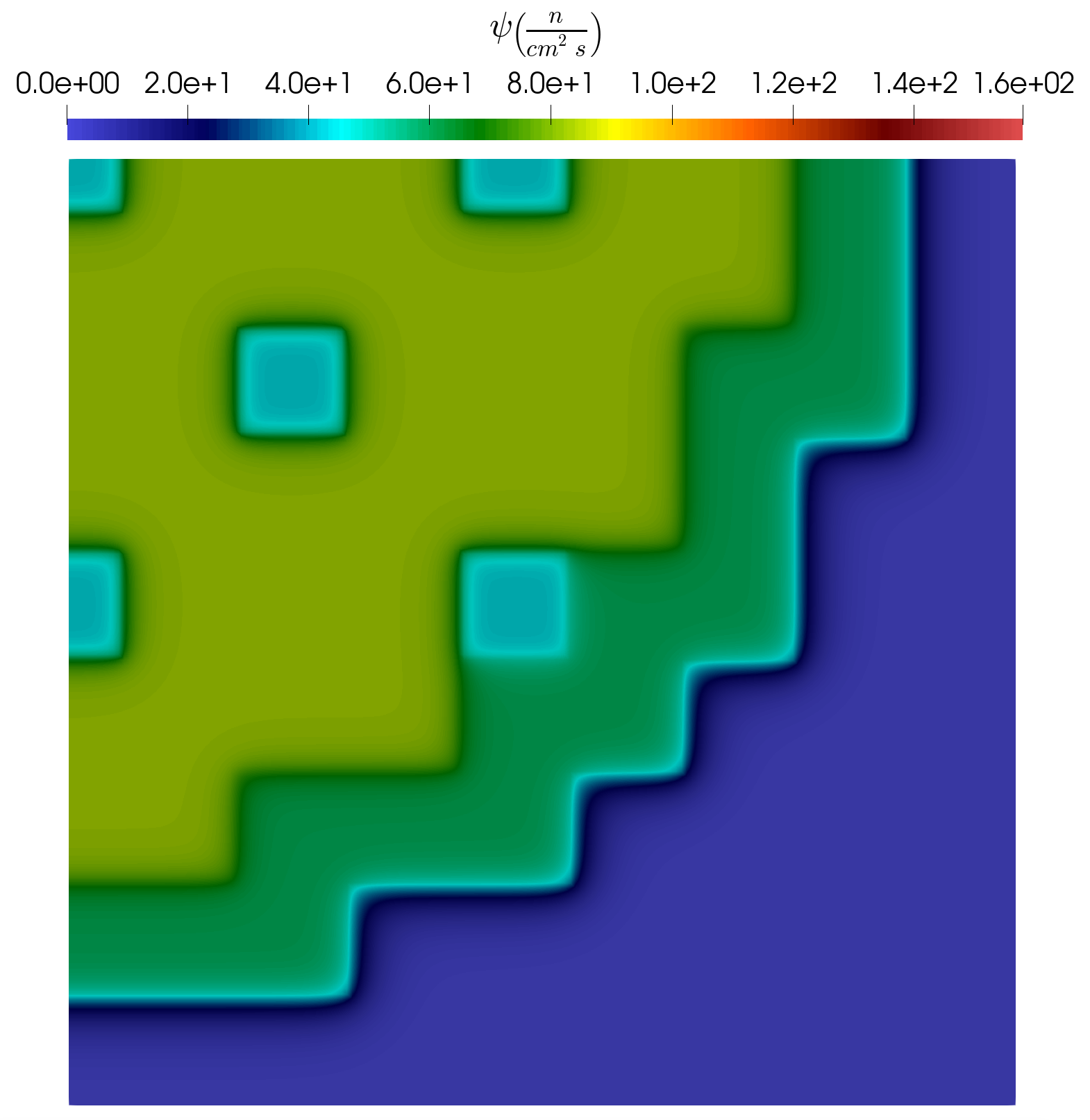
Figure 6: Snap. example #1.
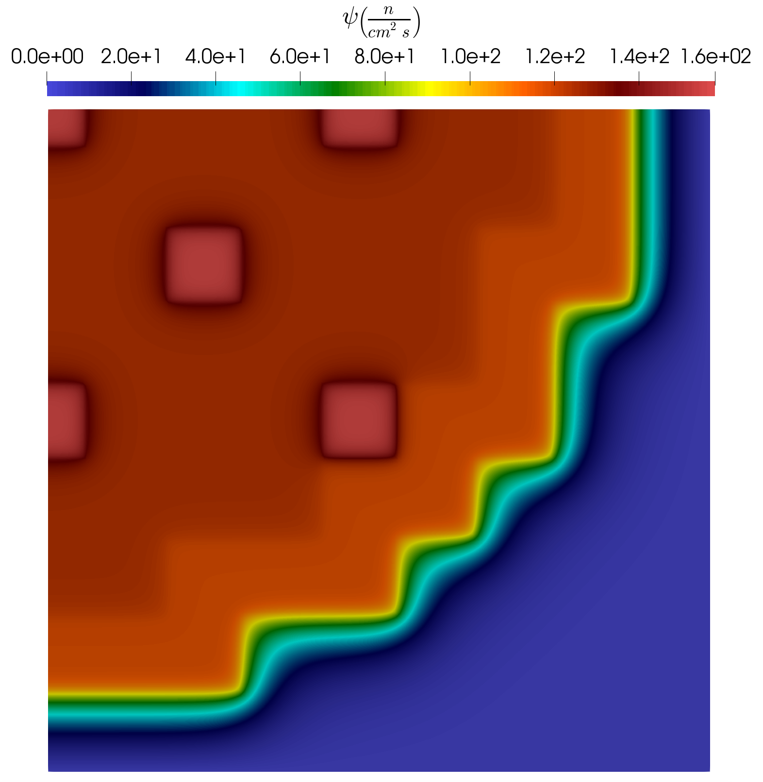
Figure 7: Snap. example #2.
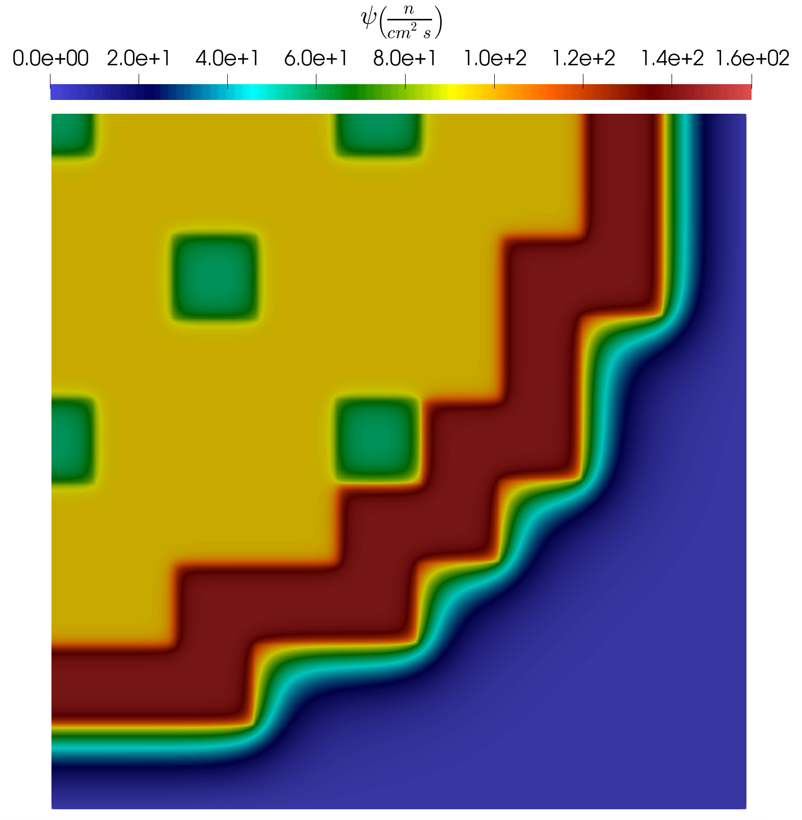
Figure 8: Snap. example #3.
After all of the snapshots are obtained, the basis functions of the reduced subspaces are extracted. In this scenario, an energy retention limit of 0.999 999 999 is used in the trainer which will keep 55 basis functions for the reduced subspace. The decay of the eigenvalues of the snapshot correlation matrix is shown in Figure 2. The reduced operators are then computed using these 55 basis functions.
Figure 2: Scree plot of the eigenvalues of the correlation matrix.
As a next step, two surrogate models are prepared using the "change_rank" and "new_ranks" parameters of PODReducedBasisSurrogate to change the size of the reduced system. The first surrogate model has 1 basis function, while the other has 8. Both models are then run on a 1000 sample test set and the nodal norms of the approximate solutions are saved. Additionally, a full-order model was executed on the same test set and the results are saved to serve as reference values. Figure 3 presents the results with the surrogate model built with 1 basis function only. It is visible that the distribution of the QoI (nodal norm) on the test set is considerably different than the reference distribution.

Figure 3: The histogram of the QoI for the full-order reference model and the surrogate built with 1 basis function.
Figure 4 shows the distribution of the QoI obtained by a surrogate with 8 basis functions. It is visible that the difference between the reference values and those from the surrogate is negligible.

Figure 4: The histogram of the QoI for the full-order reference model and the surrogate built with 8 basis function.
To see the convergence of the results from the surrogate to those of the full-order model, the surrogate model is run multiple times with different ranks and the following error indicators are computed for each sample in the test set:
Then, the maximum and average relative errors are recorder as function of the number of basis functions used. Figure 5 shows the results. It is visible that by increasing the number of basis functions, both error indicators decrease rapidly.
Figure 5: The convergence of averaged quantities of interest.
Lastly, the computation time full-order model on the test set is compared to the combined cost of training and evaluating a POD-RB surrogate model in Table 2. The test has been carried out on one processor only, not using the parallel capabilities of the MultiApp system. The results show that it is beneficial to create a POD-RB surrogate if more than 148 evaluations are needed. This assumes that the full-order evaluation time can be equally distributed among the 1000 test samples (0.779 s/sample). By dividing the training time with this number we get a critical sample number above which the generation of a surrogate model is a better alternative.
Table 2: The computation time of the full-order solutions on the test set compared to the cost of training a surrogate and evaluating it on the same test set.
| Process | Execution time (s) |
|---|---|
| Evaluation of the full-order model on the 1000 sample test set | 779.5 |
| Training a POD-RB surrogate using 100 samples | 116.2 |
| Evaluation of the POD-RB surrogate on the 1000 sample test set (4 basis functions) | 0.592 |
| Evaluation of the POD-RB surrogate on the 1000 sample test set (8 basis functions) | 0.937 |
| Evaluation of the POD-RB surrogate on the 1000 sample test set (16 basis functions) | 1.576 |
References
- Zachary M Prince and Jean C Ragusa.
Parametric uncertainty quantification using proper generalized decomposition applied to neutron diffusion.
International Journal for Numerical Methods in Engineering, 119(9):899–921, 2019.[Export]