Gaussian Process Surrogate
This example walks through the creation of a few gaussian process surrogates on a simple example system with an analytical solution for comparison. The first surrogate considers a single input parameter to be varied, which lends itself to a simple visual interpretation of the surrogate behavior. The next surrogate extends this idea to two input parameters being modeled. Lastly the full system is modeled with all input parameters, and compared to the analytical solution using sampling. It's recommended users be familiar with the basic surrogate framework, such as Creating a Surrogate Model, Training a Surrogate Model, and Evaluating a Surrogate Model.
Problem Statement
The full order model we wish to emulate with this surrogate is a one-dimensional heat conduction model with four input parameters .
When creating a surrogate using Gaussian Processes, a quantity of interest should be chosen (as opposed to attempting to model directly). In this The quantity of interest chosen for this example is the average temperature:
Input Parameters
Table 1:
| Parameter | Symbol | Normal | Uniform |
|---|---|---|---|
| Conductivity | |||
| Volumetric Heat Source | |||
| Domain Size | |||
| Right Boundary Temperature |
Analytical Solutions
This simple model problem has analytical descriptions for the field temperature and average temperature:
For that reason is chosen as the QoI to be modeled by the surrogate for this example problem. The closed form solution allows for easy comparison between the surrogate and the exact solution.
Setting up a 1D Problem
Problems with a single input variable are a good place to provide insight on Gaussian Process regression. To accomplish this three parameters of our model system are fixed , leaving the surrogate to only model the action of varying .
6 training values for were selected from and evaluated using a full model evaluation. The Gaussian Process model was fitted to these data points.
The Gaussian Process was chosen to use a SquaredExponentialCovariance covariance function, using three user selected hyperparameter settings: . To set up the training for this surrogate we require the standard Trainers block found in all surrogate models in addition to the Gaussian Process specific Covariance block. Hyperparameters vary depending on the covariance function selected, and are therefore specified in the Covariance block.
[Trainers<<<{"href": "../../../syntax/Trainers/index.html"}>>>]
  [GP_avg_trainer]
    type = GaussianProcessTrainer<<<{"description": "Provides data preperation and training for a single- or multi-output Gaussian Process surrogate model.", "href": "../../../source/trainers/GaussianProcessTrainer.html"}>>>
    execute_on<<<{"description": "The list of flag(s) indicating when this object should be executed. For a description of each flag, see https://mooseframework.inl.gov/source/interfaces/SetupInterface.html."}>>> = timestep_end
    sampler<<<{"description": "Sampler used to create predictor and response data."}>>> = train_sample
    response<<<{"description": "Reporter value of response results, can be vpp with <vpp_name>/<vector_name> or sampler column with 'sampler/col_<index>'."}>>> = results/data:avg:value
    covariance_function<<<{"description": "Name of covariance function."}>>> = 'rbf'
    standardize_params<<<{"description": "Standardize (center and scale) training parameters (x values)"}>>> = 'true' #Center and scale the training params
    standardize_data<<<{"description": "Standardize (center and scale) training data (y values)"}>>> = 'true' #Center and scale the training data
  []
[]

[Covariance<<<{"href": "../../../syntax/Covariance/index.html"}>>>]
  [rbf]
    type = SquaredExponentialCovariance<<<{"description": "Squared Exponential covariance function.", "href": "../../../source/covariances/SquaredExponentialCovariance.html"}>>>
    signal_variance<<<{"description": "Signal Variance ($\\sigma_f^2$) to use for kernel calculation."}>>> = 1 #Use a signal variance of 1 in the kernel
    noise_variance<<<{"description": "Noise Variance ($\\sigma_n^2$) to use for kernel calculation."}>>> = 1e-3 #A small amount of noise can help with numerical stability
    length_factor<<<{"description": "Length factors to use for Covariance Kernel"}>>> = '0.38971' #Select a length factor for each parameter (k and q)
  []
[]Creation of the Surrogate block follows the standard procedure laid out for other surrogate models.
[Surrogates<<<{"href": "../../../syntax/Surrogates/index.html"}>>>]
  [gauss_process_avg]
    type = GaussianProcessSurrogate<<<{"description": "Computes and evaluates Gaussian Process surrogate model.", "href": "../../../source/surrogates/GaussianProcessSurrogate.html"}>>>
    trainer<<<{"description": "The SurrogateTrainer object. If this is specified the trainer data is automatically gathered and available in this SurrogateModel object."}>>> = 'GP_avg_trainer'
  []
[]One advantage of Gaussian Process surrogates is the ability to provide an model for uncertainty. To output this data the standard EvaluateSurrogate reporter is used with specification of "evaluate_std", which also outputs the standard deviation of the surrogate at the evaluation point.
[Reporters<<<{"href": "../../../syntax/Reporters/index.html"}>>>]
  [results]
    type = StochasticReporter<<<{"description": "Storage container for stochastic simulation results coming from Reporters.", "href": "../../../source/reporters/StochasticReporter.html"}>>>
  []
  [cart_avg]
    type = EvaluateSurrogate<<<{"description": "Tool for sampling surrogate models.", "href": "../../../source/reporters/EvaluateSurrogate.html"}>>>
    model<<<{"description": "Name of surrogate models."}>>> = gauss_process_avg
    sampler<<<{"description": "Sampler to use for evaluating surrogate models."}>>> = cart_sample
    evaluate_std<<<{"description": "Whether or not to evaluate standard deviation associated with each sample, a single entry will use it for every model. Warning: not every model can compute standard deviation."}>>> = 'true'
    parallel_type<<<{"description": "This parameter will determine how the stochastic data is gathered. It is common for outputting purposes that this parameter be set to ROOT, otherwise, many files will be produced showing the values on each processor. However, if there are lot of samples, gathering on root may be memory restrictive."}>>> = ROOT
    execute_on<<<{"description": "The list of flag(s) indicating when this object should be executed. For a description of each flag, see https://mooseframework.inl.gov/source/interfaces/SetupInterface.html."}>>> = final
  []
  [train_avg]
    type = EvaluateSurrogate<<<{"description": "Tool for sampling surrogate models.", "href": "../../../source/reporters/EvaluateSurrogate.html"}>>>
    model<<<{"description": "Name of surrogate models."}>>> = gauss_process_avg
    sampler<<<{"description": "Sampler to use for evaluating surrogate models."}>>> = train_sample
    evaluate_std<<<{"description": "Whether or not to evaluate standard deviation associated with each sample, a single entry will use it for every model. Warning: not every model can compute standard deviation."}>>> = 'true'
    parallel_type<<<{"description": "This parameter will determine how the stochastic data is gathered. It is common for outputting purposes that this parameter be set to ROOT, otherwise, many files will be produced showing the values on each processor. However, if there are lot of samples, gathering on root may be memory restrictive."}>>> = ROOT
    execute_on<<<{"description": "The list of flag(s) indicating when this object should be executed. For a description of each flag, see https://mooseframework.inl.gov/source/interfaces/SetupInterface.html."}>>> = final
  []
[]The Gaussian Process surrogate model can only be evaluated at discrete points in the parameter space, so if we wish to visualize the response model fine sampling is required. To accomplish this sampling a CartesianProductSampler evaluates the model for 100 evenly spaced values in . This sampling is plotted below in Figure 1 (space between the 100 sampled points are filled by simple linear interpolation, so strictly speaking the plot is not exactly the model)
[Samplers<<<{"href": "../../../syntax/Samplers/index.html"}>>>]
  [train_sample]
    type = MonteCarlo<<<{"description": "Monte Carlo Sampler.", "href": "../../../source/samplers/MonteCarloSampler.html"}>>>
    num_rows<<<{"description": "The number of rows per matrix to generate."}>>> = 6
    distributions<<<{"description": "The distribution names to be sampled, the number of distributions provided defines the number of columns per matrix."}>>> = 'q_dist'
    execute_on<<<{"description": "The list of flag(s) indicating when this object should be executed. For a description of each flag, see https://mooseframework.inl.gov/source/interfaces/SetupInterface.html."}>>> = PRE_MULTIAPP_SETUP
  []
  [cart_sample]
    type = CartesianProduct<<<{"description": "Provides complete Cartesian product for the supplied variables.", "href": "../../../source/samplers/CartesianProductSampler.html"}>>>
    linear_space_items<<<{"description": "A list of triplets, each item should include the min, step size, and number of steps."}>>> = '9000 20 100'
    execute_on<<<{"description": "The list of flag(s) indicating when this object should be executed. For a description of each flag, see https://mooseframework.inl.gov/source/interfaces/SetupInterface.html."}>>> = initial
  []
[]
Figure 1: Surrogate model for 1D problem using fixed (user specified) hyperparameters.
Figure 1 demonstrates some basic principles of the gaussian process surrogate for this covariance function. Near training points (red + markers), the uncertainty in the model trends towards the measurement noise . The model function is smooth and infinitely differentiable. As we move away from the data points the model tends to just predict the mean of the training data, particularly noticeable in the extrapolation regions of the graph.
However, given that in this scenario we know the model should be a simple linear fit, we may conclude that this fit should be better. To achieve a better fit the model needs to be adjusted, specifically better hyperparameters for the covariance function likely need to be tested. For many hyperparameters this can be accomplished automatically by the system. To enable this specify the tuned hyperparameters using "tune_parameters" in the trainer. Tuning bounds can be placed using "tuning_min" and "tuning_max".
[Trainers<<<{"href": "../../../syntax/Trainers/index.html"}>>>]
  [GP_avg_trainer]
    type = GaussianProcessTrainer<<<{"description": "Provides data preperation and training for a single- or multi-output Gaussian Process surrogate model.", "href": "../../../source/trainers/GaussianProcessTrainer.html"}>>>
    execute_on<<<{"description": "The list of flag(s) indicating when this object should be executed. For a description of each flag, see https://mooseframework.inl.gov/source/interfaces/SetupInterface.html."}>>> = timestep_end
    response<<<{"description": "Reporter value of response results, can be vpp with <vpp_name>/<vector_name> or sampler column with 'sampler/col_<index>'."}>>> = results/data:avg:value
    covariance_function<<<{"description": "Name of covariance function."}>>> = 'rbf'
    standardize_params<<<{"description": "Standardize (center and scale) training parameters (x values)"}>>> = 'true' #Center and scale the training params
    standardize_data<<<{"description": "Standardize (center and scale) training data (y values)"}>>> = 'true' #Center and scale the training data
    sampler<<<{"description": "Sampler used to create predictor and response data."}>>> = train_sample
    tune_parameters<<<{"description": "Select hyperparameters to be tuned"}>>> = 'rbf:signal_variance rbf:length_factor'
    tuning_min<<<{"description": "Minimum allowable tuning value"}>>> = ' 1e-9 1e-9'
    tuning_max<<<{"description": "Maximum allowable tuning value"}>>> = ' 1e16  1e16'
    num_iters<<<{"description": "Tolerance value for Adam optimization"}>>> = 10000
    batch_size<<<{"description": "The batch size for Adam optimization"}>>> = 6
    learning_rate<<<{"description": "The learning rate for Adam optimization"}>>> = 0.0005
    show_every_nth_iteration<<<{"description": "Switch to show Adam optimization loss values at every nth step. If 0, nothing is showed."}>>> = 1
  []
[]

[Covariance<<<{"href": "../../../syntax/Covariance/index.html"}>>>]
  [rbf]
    type = SquaredExponentialCovariance<<<{"description": "Squared Exponential covariance function.", "href": "../../../source/covariances/SquaredExponentialCovariance.html"}>>>
    signal_variance<<<{"description": "Signal Variance ($\\sigma_f^2$) to use for kernel calculation."}>>> = 1 #Use a signal variance of 1 in the kernel
    noise_variance<<<{"description": "Noise Variance ($\\sigma_n^2$) to use for kernel calculation."}>>> = 1e-3 #A small amount of noise can help with numerical stability
    length_factor<<<{"description": "Length factors to use for Covariance Kernel"}>>> = '0.38971' #Select a length factor for each parameter (k and q)
  []
[]To demonstrate the importance of hyperparameter tuning, the same data set was then used to train a surrogate with hyperparameter auto-tuning enabled. In this mode the system attempts to learn an optimal hyperparameter configuration to maximize the likelihood of observing the data from the fitted model. The results shown in Figure 2 is a nearly linear fit, with very little uncertainty in the fit, which is what we expect from the analytical form.

Figure 2: Surrogate model for 1D problem using tuned hyperparameters.
Inspection of the final hyperparameter values after tuning gives , the significant increase in the length scale is a primary factor in the improved fit.
Setting up a 2D Problem
Next the idea is extended to two input dimensions and attempt to model the QoI behavior due to varying and , while fixing values of .
Due to the increased dimensionality, 50 training samples were selected from and . An extra hyperparameter is also added to the set of hyperparameters to be tuned.
[Samplers<<<{"href": "../../../syntax/Samplers/index.html"}>>>]
  [train_sample]
    type = MonteCarlo<<<{"description": "Monte Carlo Sampler.", "href": "../../../source/samplers/MonteCarloSampler.html"}>>>
    num_rows<<<{"description": "The number of rows per matrix to generate."}>>> = 50
    distributions<<<{"description": "The distribution names to be sampled, the number of distributions provided defines the number of columns per matrix."}>>> = 'k_dist q_dist'
    execute_on<<<{"description": "The list of flag(s) indicating when this object should be executed. For a description of each flag, see https://mooseframework.inl.gov/source/interfaces/SetupInterface.html."}>>> = PRE_MULTIAPP_SETUP
  []
  [cart_sample]
    type = CartesianProduct<<<{"description": "Provides complete Cartesian product for the supplied variables.", "href": "../../../source/samplers/CartesianProductSampler.html"}>>>
    linear_space_items<<<{"description": "A list of triplets, each item should include the min, step size, and number of steps."}>>> = '1 0.09 10
                          9000 20 10 '
    execute_on<<<{"description": "The list of flag(s) indicating when this object should be executed. For a description of each flag, see https://mooseframework.inl.gov/source/interfaces/SetupInterface.html."}>>> = initial
  []
[]

[Trainers<<<{"href": "../../../syntax/Trainers/index.html"}>>>]
  [GP_avg_trainer]
    type = GaussianProcessTrainer<<<{"description": "Provides data preperation and training for a single- or multi-output Gaussian Process surrogate model.", "href": "../../../source/trainers/GaussianProcessTrainer.html"}>>>
    execute_on<<<{"description": "The list of flag(s) indicating when this object should be executed. For a description of each flag, see https://mooseframework.inl.gov/source/interfaces/SetupInterface.html."}>>> = timestep_end
    covariance_function<<<{"description": "Name of covariance function."}>>> = 'rbf'
    standardize_params<<<{"description": "Standardize (center and scale) training parameters (x values)"}>>> = 'true' #Center and scale the training params
    standardize_data<<<{"description": "Standardize (center and scale) training data (y values)"}>>> = 'true' #Center and scale the training data
    sampler<<<{"description": "Sampler used to create predictor and response data."}>>> = train_sample
    response<<<{"description": "Reporter value of response results, can be vpp with <vpp_name>/<vector_name> or sampler column with 'sampler/col_<index>'."}>>> = results/data:avg:value
    tune_parameters<<<{"description": "Select hyperparameters to be tuned"}>>> = 'rbf:signal_variance rbf:length_factor'
    tuning_min<<<{"description": "Minimum allowable tuning value"}>>> = '1e-9 1e-9'
    tuning_max<<<{"description": "Maximum allowable tuning value"}>>> = '1e16  1e16'
    batch_size<<<{"description": "The batch size for Adam optimization"}>>> = 50
    num_iters<<<{"description": "Tolerance value for Adam optimization"}>>> = 5000
    learning_rate<<<{"description": "The learning rate for Adam optimization"}>>> = 5e-3
  []
[]

[Covariance<<<{"href": "../../../syntax/Covariance/index.html"}>>>]
  [rbf]
    type = SquaredExponentialCovariance<<<{"description": "Squared Exponential covariance function.", "href": "../../../source/covariances/SquaredExponentialCovariance.html"}>>>
    signal_variance<<<{"description": "Signal Variance ($\\sigma_f^2$) to use for kernel calculation."}>>> = 1 #Use a signal variance of 1 in the kernel
    noise_variance<<<{"description": "Noise Variance ($\\sigma_n^2$) to use for kernel calculation."}>>> = 1e-3 #A small amount of noise can help with numerical stability
    length_factor<<<{"description": "Length factors to use for Covariance Kernel"}>>> = '0.38971 0.38971' #Select a length factor for each parameter (k and q)
  []
[]As was done in the 1D case above, first the surrogate was fitted using fixed hyperparameters . The QoI surface is shown in Figure 3, with the color map corresponding to the surrogate model's uncertainty at that point. As was the case in the 1D mode, uncertainty is highest at points furthest from training data points, and the overall response deviates strongly from the expected behavior predicted.

Figure 3: Surrogate model for 2D problem using fixed hyperparameters.
Hyperparameter tuning is then enabled by setting "tune_parameters". Figure 4 shows the fit with automatically tuned hyperparameters using the same data set. This results in a fit that much better captures the nature of the QoI response, with "high" uncertainty occurring primarily in extrapolation zones.

Figure 4: Surrogate model for 2D problem using tuned hyperparameters.
Full 4D Problem
This idea is then extended naturally to the full problem in which the parameter set is modeled. Training occurs using training points in. Evaluation occurs by sampling the surrogate times with perturbed inputs, with results shown in histogram form in Figure 5. While the evaluation points are sampled from the normal distribution in Table 1,the training data points are sampled from the uniform distributions. Sampling the training data from the normal distribution can result in an imbalance of data points near the mean, causing poor performance in outlying regions. The training and evaluation inputs are (contrib/moose/modules/stochastic_tools/examples/surrogates/gaussian_process/GP_normal_mc.i) and (contrib/moose/modules/stochastic_tools/examples/surrogates/gaussian_process/GP_normal.i) respectively.
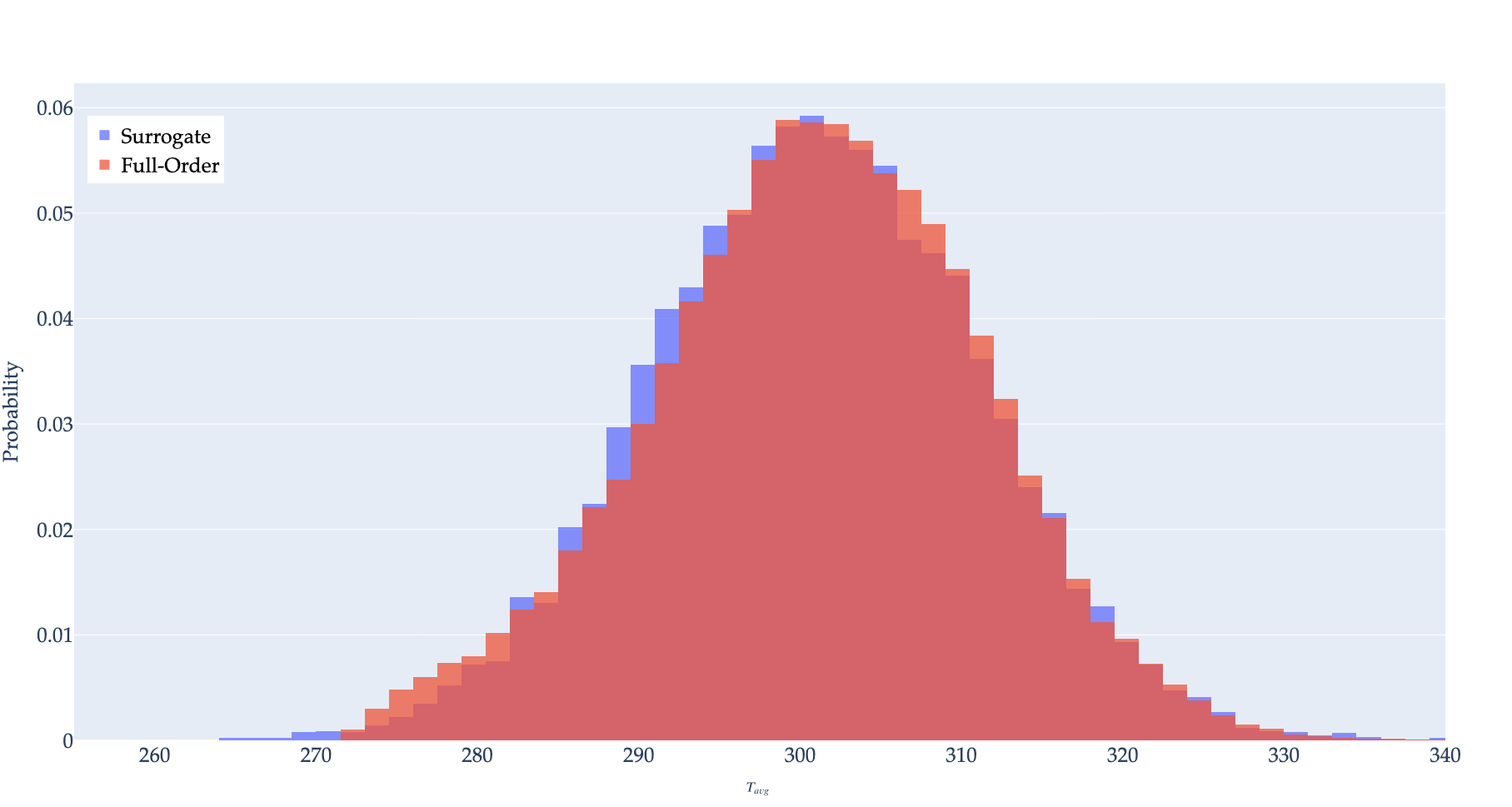
Figure 5: Histogram of samples of surrogate compared to exact.
To showcase more optimization options available in GaussianProcessTrainer, we used Adam for fitting the length scales and signal variance in this process. The parameters for Adam (number of iterations, learning rate, etc.) can be set using the following syntax:
[Trainers<<<{"href": "../../../syntax/Trainers/index.html"}>>>]
  [GP_avg]
    type = GaussianProcessTrainer<<<{"description": "Provides data preperation and training for a single- or multi-output Gaussian Process surrogate model.", "href": "../../../source/trainers/GaussianProcessTrainer.html"}>>>
    execute_on<<<{"description": "The list of flag(s) indicating when this object should be executed. For a description of each flag, see https://mooseframework.inl.gov/source/interfaces/SetupInterface.html."}>>> = timestep_end
    covariance_function<<<{"description": "Name of covariance function."}>>> = 'rbf'
    standardize_params<<<{"description": "Standardize (center and scale) training parameters (x values)"}>>> = 'true' #Center and scale the training params
    standardize_data<<<{"description": "Standardize (center and scale) training data (y values)"}>>> = 'true' #Center and scale the training data
    sampler<<<{"description": "Sampler used to create predictor and response data."}>>> = sample
    response<<<{"description": "Reporter value of response results, can be vpp with <vpp_name>/<vector_name> or sampler column with 'sampler/col_<index>'."}>>> = results/data:avg:value
    tune_parameters<<<{"description": "Select hyperparameters to be tuned"}>>> = 'rbf:signal_variance rbf:length_factor'
    tuning_min<<<{"description": "Minimum allowable tuning value"}>>> = ' 1e-9 1e-3'
    tuning_max<<<{"description": "Maximum allowable tuning value"}>>> = ' 100  100'
    num_iters<<<{"description": "Tolerance value for Adam optimization"}>>> = 200
    learning_rate<<<{"description": "The learning rate for Adam optimization"}>>> = 0.005
  []
[]