Bayesian Uncertainty Quantification (UQ) on a 1D Diffusion Problem

This example demonstrates how to infer unknown model parameters given experimental observations. Uncertainties of the model parameters are inversely quantified through the Bayesian framework, which makes use of samplers including IndependentGaussianMH (Independent Gaussian Metropolis-Hastings), AffineInvariantStretchSampler or AffineInvariantDES (AffineInvariantDifferential).

Overview of Bayesian UQ

In general, assume a computational model $\mathcal{M}(\theta)$ , where $\theta$ are unknown model parameters. Original belief about the unknown parameters, described by the prior distribution $f(\pmb{\theta}, \sigma)$ , is usually subject to large uncertainties. Given experimental measurements $\pmb{\mathcal{D}}$ of the computational model at specific configuration conditions $\pmb{\Theta}$ , updated knowledge about the model parameters $f(\pmb{\theta}, \sigma | \pmb{\Theta}, \mathcal{M}, \pmb{\mathcal{D}})$ can be obtained by the Bayes' theorem:

f(\pmb{\theta}, \sigma | \pmb{\Theta}, \mathcal{M}, \pmb{\mathcal{D}}) \propto \mathcal{L}(\pmb{\theta}, \sigma | \pmb{\Theta}, \mathcal{M}, \pmb{\mathcal{D}})~f(\pmb{\theta}, \sigma)

where $\mathcal{L}(\pmb{\theta}, \sigma | \pmb{\Theta}, \mathcal{M}, \pmb{\mathcal{D}})$ is the Likelihood function. Gaussian and TruncatedGaussian distributions are the most popular choices for the likelihood function. Variance of the Guassian or truncated Gaussian, which describes the sum of the model discrepancy and measurement error (referred to as $\sigma$ term herein), can be either fixed a priori or inferred from the experimental measurements $\pmb{\mathcal{D}}$ . The goal of Bayesian UQ is to infer the unknown parameters $\pmb{\theta}$ (and $\sigma$ if needed) given experimental measurements $\pmb{\mathcal{D}}$ , i.e., the posterior distributions $f(\pmb{\theta}, \sigma | \pmb{\Theta}, \mathcal{M}, \pmb{\mathcal{D}})$ .

The code architecture for performing Markov Chain Monte Carlo (MCMC) sampling in a parallelized fashion is presented in Figure 1. There are three steps for performing the sampling: proposal, model evaluation, and decision making. These three steps and the respective code objects are discussed below:

Proposals: The proposals are made using the user-defined specific MCMC Samplers object which derives from the MCMC base class PMCMCBase. The specific MCMC sampler can be any variant of either serial or parallel MCMC techniques. In total, the MCMC sampler object proposes $P$ proposals which are subsequently sent to the MultiApps system.
Model evaluation: The MultiApps system executes the models for each of the parallel proposals. In total, there will be $P \times N$ model evaluations, where $N$ is the number of experimental configurations. MultiApps is responsible for distributing these jobs across a given set of processors.
Decision making: The model outputs from the MultiApps system are gathered by a Reporters object to compute the likelihood function. Then, the acceptance probabilities are computed for the $P$ parallel proposals and accept/reject decisions are made. The information of accepted samples is sent to the MCMC sampler object to influence the next set of $P$ proposals.

The above three steps are repeated for a user-specified number of times.

Figure 1: Code architecture for parallelized MCMC sampling in MOOSE for performing Bayesian UQ (Dhulipala et al. (2023)).

Problem Statement

This tutorial demonstrates the application of Bayesian UQ on a 1D transient diffusion problem with Dirichlet boundary conditions on each end of the domain:

\frac{\partial u}{\partial t} - \frac{\partial^2 u}{\partial x^2} = 0 \quad x \in [0,L],

u(t=0, x) = 0

\begin{aligned} u(t, x=0) = u_{\mathrm{left}} \\ u(t, x=L) = u_{\mathrm{right}} \end{aligned}

where $u(t, x)$ defines the solution field. The experiments measure the average solution field across the entire domain length $L$ at the end of time $T$ . Experimental measurements are pre-generated at eight configuration points $L=1.0, 2.0, ..., 8.0$ . A Gaussian noise with standard deviation of 0.05 is added to simulate the measurement error. The goal is to infer the lefthandside and righthandside Dirichlet boundary conditions, i.e., $u(x=0)$ and $u(x=L)$ , referred to as $u_{\mathrm{left}}$ and $u_{\mathrm{right}}$ for conciseness. It is worth pointing out that the $\sigma$ term, which is the variance of the sum of the experimental measurement and model deviations, can also be inferred during the Bayesian UQ process. This tutorial will first demonstrate the inference of true boundary values by assuming a fixed variance term for the experimental error, followed by the inference of the boundary values together with variance term.

Inferring Calibration Parameters Only (Fixed $\sigma$ Term)

Sub-Application Input

The problem defined above, with respect to the MultiApps system, is a sub-application. The complete input file for the problem is provided in Listing 1.

Listing 1: Complete input file for executing the transient diffusion problem.

left_bc = 0.13508909593042528
right_bc = -1.5530467809139854
mesh1 = 1

param1 = '${fparse left_bc}'
param2 = '${fparse right_bc}'
param3 = '${fparse mesh1}'

[Mesh]
  type = GeneratedMesh
  dim = 2
  xmax = ${param3}
  xmin = 0
  ymax = 1
  ymin = 0
  nx = 10
  ny = 10
[]

[Variables]
  [u]
  []
[]

[Kernels]
  [diff]
    type = Diffusion
    variable = u
  []
  [time]
    type = TimeDerivative
    variable = u
  []
[]

[BCs]
  [left]
    type = DirichletBC
    variable = u
    boundary = left
    value = ${param1} # Actual = 0.15
  []
  [right]
    type = DirichletBC
    variable = u
    boundary = right
    value = ${param2} # Actual = -1.5
  []
[]

[Postprocessors]
  [average]
    type = ElementAverageValue
    variable = u
  []
[]

[Executioner]
  type = Transient
  num_steps = 5
  dt = 0.1
  solve_type = PJFNK
  petsc_options_iname = '-pc_type -pc_hypre_type'
  petsc_options_value = 'hypre boomeramg'
[]

[Outputs]
  console = 'false'
[]

Main Input

The main application, with respect to the MultiApps system, is the driver of the stochastic simulations. The main input does not perform a solve itself, couples with the sub-application for the full stochastic analysis. Details of each individual input section will is explained in details as follows.

The StochasticTools block is defined at the beginning of the main application to automatically create the necessary objects for running a stochastic analysis.

[StochasticTools]
[]

The Distributions block is used to define the prior distributions for the two stochastic boundary conditions. In this example, the two stochastic boundary conditions are assumed to follow normal distributions

[Distributions]
  [left]
    type = Normal
    mean = 0.0
    standard_deviation = 1.0
  []
  [right]
    type = Normal
    mean = 0.0
    standard_deviation = 1.0
  []
[]

A Likelihoods object is created to specify the type of likelihood function used in the analysis.

A Gaussian-type log-likelihood function is used in the current analysis, as specified by type = Gaussian and log_likelihood = true.
The noise term defines the experimental noise plus model deviations against experiments. Scale of the Gaussian distribution is fixed to a constant value of 0.05 through the noise_specified term, as will be explained next in the Reporters block. Note that this term can be inferred
The file_name argument takes in a CSV file that contains experimental values. In this example, the exp_0.05.csv file contains 8 independent experimental measurements, which are the sum of pre-simulated solution and a Gaussian noise with standard deviation of 0.05.

[Likelihood]
  [gaussian]
    type = Gaussian
    noise = 'noise_specified/noise_specified'
    file_name = 'exp_0_05.csv'
    log_likelihood = true
  []
[]

In the Samplers block, AffineInvariantDES is used to sample the left and right boundary conditions according to the parallelized Markov chain Monte Carlo method at certain configuration conditions.

prior_distributions takes in the pre-defined prior distributions of the parameters to be calibrated.
num_parallel_proposals specifies the number of proposals to make and corresponding sub-applications executed in parallel.
initial_values defines the starting values of the parameters to be calibrated.
file_name takes in a CSV file that contains the configuration values. In this example, the confg.csv file contains 8 configuration values $L=1.0, 2.0, ..., 8.0$ .

[Samplers]
  [sample]
    type = AffineInvariantDES
    prior_distributions = 'left right'
    num_parallel_proposals = 5
    file_name = 'confg.csv'
    execute_on = PRE_MULTIAPP_SETUP
    seed = 2547
    initial_values = '0.1 0.1'
    previous_state = 'mcmc_reporter/inputs'
    previous_state_var = 'mcmc_reporter/variance'
  []
[]

In the MultiApps block, a SamplerFullSolveMultiApp object is defined to create and run a sub-application for each sample provided by the sampler object. More specifically, a full-solve type sub-application is executed for each row of the Sampler matrix.

[MultiApps]
  [sub]
    type = SamplerFullSolveMultiApp
    input_files = sub.i
    sampler = sample
  []
[]

Under the Transfers block, SamplerReporterTransfer is utilized to transfer data from Reporters on the sub-application to a StochasticReporter on the main application. In this example, the value of a postprocessor named average, as defined in the sub-application, is transferred to a StochasticReporter named constant in the main application.

[Transfers]
  [reporter_transfer]
    type = SamplerReporterTransfer
    from_reporter = 'average/value'
    stochastic_reporter = 'constant'
    from_multi_app = sub
    sampler = sample
  []
[]

The Controls block makes use of MultiAppSamplerControl to pass command line arguments from the main application to the sub-applications. In this example, three arguments are passed from the main application to the sub-applications, i.e.,

left_bc: the Dirichlet boundary condition at the lefthandside of the domain.
right_bc: the Dirichlet boundary condition at the righthandside of the domain.
mesh1: the domain length, which is controlled by the configuration parameters in the Samplers block.

[Controls]
  [cmdline]
    type = MultiAppSamplerControl
    multi_app = sub
    sampler = sample
    param_names = 'left_bc right_bc mesh1'
  []
[]

Then, the Reporters section defines Reporter objects for data transfer in the MultiApps system.

The constant reporter of type StochasticReporter serves as a storage container for stochastic simulation results coming from the sub-application.
noise_specified makes use of the ConstantReporter reporter to generate a constant value, which is used for the variance term in the experimental error in this example. The value is specified to be 0.05 as defined in real_values.
mcmc_reporter is of type AffineInvariantDES which makes the decision whether or not to accept a proposal generated by the parallel Markov chain Monte Carlo algorithms. It takes in a likelihood function likelihoods, a sampler, and the model output from the sub-application output_value. In this example, output_value = constant/reporter_transfer:average:value means that the model output from the sub-application is obtained by a reporter named constant, which interacts with the reporter reporter_transfer to transfer the average solution field.

[Reporters]
  [constant]
    type = StochasticReporter
  []
  [noise_specified]
    type = ConstantReporter
    real_names = 'noise_specified'
    real_values = '0.05'
  []
  [mcmc_reporter]
    type = AffineInvariantDifferentialDecision
    output_value = constant/reporter_transfer:average:value
    sampler = sample
    likelihoods = 'gaussian'
  []
[]

Available Sampling Algorithms

Currently, multiple parallel MCMC samplers have been implemented in stochastic tools module, including IndependentGaussianMH, AffineInvariantStretchSampler, and AffineInvariantDES. The above example is demonstrated on AffineInvariantDES. Switching to a different MCMC sampler only requires minor changes in the Samplers block and the Reporters block in the main input file, while the input syntax for the sub-application remains the same. Three available MCMC samplers are explained below respectively:

IndependentGaussianMH(IMH): Performs Metropolis-Hastings MCMC sampling with independent Gaussian proposals. Under the Samplers block, std_prop specifies the standard deviations of the independent Gaussian proposals for making the next proposal. seed_inputs takes in a reporter named mcmc_reporter which reports seed inputs values for the next proposals. The mcmc_reporter is defined under the Reporters block of type IndependentMHDecision, which performs decision making for independent Metropolis-Hastings MCMC (Calderhead, 2014).

[Samplers]
  [sample]
    type = IndependentGaussianMH
    prior_distributions = 'left right'
    # previous_state = 'mcmc_reporter/inputs'
    num_parallel_proposals = 5
    file_name = 'confg.csv'
    execute_on = PRE_MULTIAPP_SETUP
    seed = 2547
    std_prop = '0.05 0.05'
    initial_values = '0.1 0.1'
    seed_inputs = 'mcmc_reporter/seed_input'
  []
[]

[Reporters]
  [constant]
    type = StochasticReporter
  []
  [noise_specified]
    type = ConstantReporter
    real_names = 'noise_specified'
    real_values = '0.05'
  []
  [mcmc_reporter]
    type = IndependentMHDecision
    output_value = constant/reporter_transfer:average:value
    sampler = sample
    likelihoods = 'gaussian'
  []
[]

AffineInvariantStretchSampler(SS): Performs affine-invariant ensemble MCMC with stretch sampler (Goodman and Weare, 2010; Shields et al., 2021). Different from other samplers, it takes in two reporters to access the mean and variance of the previous state of all the walkers (previous_state). By default, the walkers take a step size of 0.2 in the stretch sampler. Correspondingly, an mcmc_reporter of type AffineInvariantStretchDecision need be defined in the Reporters block for decision making.

[Samplers]
  [sample]
    type = AffineInvariantStretchSampler
    prior_distributions = 'left right'
    num_parallel_proposals = 5
    file_name = 'confg.csv'
    execute_on = PRE_MULTIAPP_SETUP
    seed = 2547
    initial_values = '0.1 0.1'
    previous_state = 'mcmc_reporter/inputs'
    previous_state_var = 'mcmc_reporter/variance'
  []
[]

[Reporters]
  [constant]
    type = StochasticReporter
  []
  [noise_specified]
    type = ConstantReporter
    real_names = 'noise_specified'
    real_values = '0.05'
  []
  [mcmc_reporter]
    type = AffineInvariantStretchDecision
    output_value = constant/reporter_transfer:average:value
    sampler = sample
    likelihoods = 'gaussian'
  []
[]

AffineInvariantDES(DES): Performs affine-invariant ensemble MCMC with differential sampler (Braak, 2006; Nelson et al., 2013). Similar to the stretch sampler, the evolution sampler requires two reporters to access the mean and variance of the previous state of all the walkers (previous_state). Correspondingly, an mcmc_reporter of type AffineInvariantDifferentialDecision need be defined in the Reporters block for decision making.

[Samplers]
  [sample]
    type = AffineInvariantDES
    prior_distributions = 'left right'
    num_parallel_proposals = 5
    file_name = 'confg.csv'
    execute_on = PRE_MULTIAPP_SETUP
    seed = 2547
    initial_values = '0.1 0.1'
    previous_state = 'mcmc_reporter/inputs'
    previous_state_var = 'mcmc_reporter/variance'
  []
[]

[Reporters]
  [constant]
    type = StochasticReporter
  []
  [noise_specified]
    type = ConstantReporter
    real_names = 'noise_specified'
    real_values = '0.05'
  []
  [mcmc_reporter]
    type = AffineInvariantDifferentialDecision
    output_value = constant/reporter_transfer:average:value
    sampler = sample
    likelihoods = 'gaussian'
  []
[]

Inferring Both Calibration Parameters and the Variance Term

In addition to inferring the model parameters, the variance term can also be inferred at the same time. Both the differential evolution sampler AffineInvariantDES or stretch sampler AffineInvariantStretchSampler can be used for this purpose. Changes in the following blocks are necessary in the main input file.

A prior distribution need be defined under the Distributions block. In this example, a uniform distribution with wide uncertainty range is specified for the variance term as a conservative assumption.

[Distributions]
  [left]
    type = Normal
    mean = 0.0
    standard_deviation = 1.0
  []
  [right]
    type = Normal
    mean = 0.0
    standard_deviation = 1.0
  []
  [variance]
    type = Uniform
    lower_bound = 0.0
    upper_bound = 0.5
  []
[]

In the definition of the Likelihood block, the variance term for the Gaussian likelihood function is returned by a reporter named mcmc_reporter, which is defined in the Reporters block of type AffineInvariantDifferentialDecision.

[Likelihood]
  [gaussian]
    type = Gaussian
    noise = 'mcmc_reporter/noise'
    file_name = 'exp_0_05.csv'
    log_likelihood = true
  []
[]

[Reporters]
  [constant]
    type = StochasticReporter
  []
  [mcmc_reporter]
    type = AffineInvariantDifferentialDecision
    output_value = constant/reporter_transfer:average:value
    sampler = sample
    likelihoods = 'gaussian'
  []
[]

Finally, in the Samplers block, the AffineInvariantDES sampler takes in the prior distribution of the variance term via the prior_variance argument. In this example, the prior distribution of the variance term has been defined in variance under the Distributions block.

[Samplers]
  [sample]
    type = AffineInvariantDES
    prior_distributions = 'left right'
    num_parallel_proposals = 5
    file_name = 'confg.csv'
    execute_on = PRE_MULTIAPP_SETUP
    seed = 2547
    initial_values = '0.1 0.1'
    previous_state = 'mcmc_reporter/inputs'
    previous_state_var = 'mcmc_reporter/variance'
    prior_variance = 'variance'
  []
[]

Result and Analysis

The output JSON file contains samples across different processors at different timesteps. Practically, all MCMC samples are generated with serial auto-correlations. Therefore, it is essential to diagnose the sample auto-correlation for predictable UQ quality. Two primary diagnostics are presented here for analyzing the sample quality: the integrated auto-correlation time ( $\tau_p$ ), and the effective sample size (ESS) Dhulipala et al. (2023). $\tau_p$ describes the interval after which a sample can be considered independent given a current sample index, and ESS describes the number of "effective" samples after taking into consideration the sample auto-correlation. To obtain "independent" samples from the Markov chains, the first 100 samples are discarded for "burn-in", with the remaining samples thinned by $\tau_p/2$ . The ESS of the generated samples are calculated based on the thinned samples. As presented in Table 1, $\tau_p$ for IMH, SS and DES decreases, and ESS for the three algorithms increases correspondingly, indicating the best sampling qualify by DES, followed by SS, then IMH.

Table 1: Integrated autocorrelation time ( $\tau_p$ ) and effective sample size (ESS) when inferring model parameters

Algorithm	$\tau_p$	ESS
IMH	123.908	9.528
SS	41.779	46.719
DES	11.217	676.547

When inferring only the boundary conditions, all three samplers are applied, with 1,000 serial steps simulated with 5 parallel proposals per step. Figure 2 shows the posterior distributions of the calibration parameters $u_{\mathrm{left}}$ and $u_{\mathrm{right}}$ . A strong linearity is observed for the two parameters as would be expected from the underlying physics. The IMH samples appear to be extremely localized compared to DES. The SS samples are almost as good as samples generated by DES in terms of exploring the parameter space. The DES samples are the best from this aspect. More detailed posterior distributions are presented in Figure 3 for all three algorithms IMH, SS and DES. It is generally observed that the posteriors using IMH are restricted in the parameter space. Whereas, the posteriors for both SS and DES are spread across the parameter space and look comparable to each other. This can be observed by comparing Figure 3b and Figure 3c for the posterior of $u_{\mathrm{left}}$ , and Figure 3e and Figure 3f for the posterior of $u_{\mathrm{right}}$ .

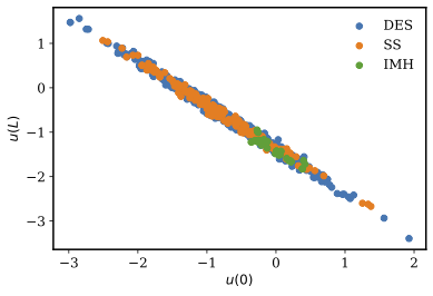
Figure 2: Scatter plot of the samples from IMH, SS, and DES samplers when only inferring the model parameters.

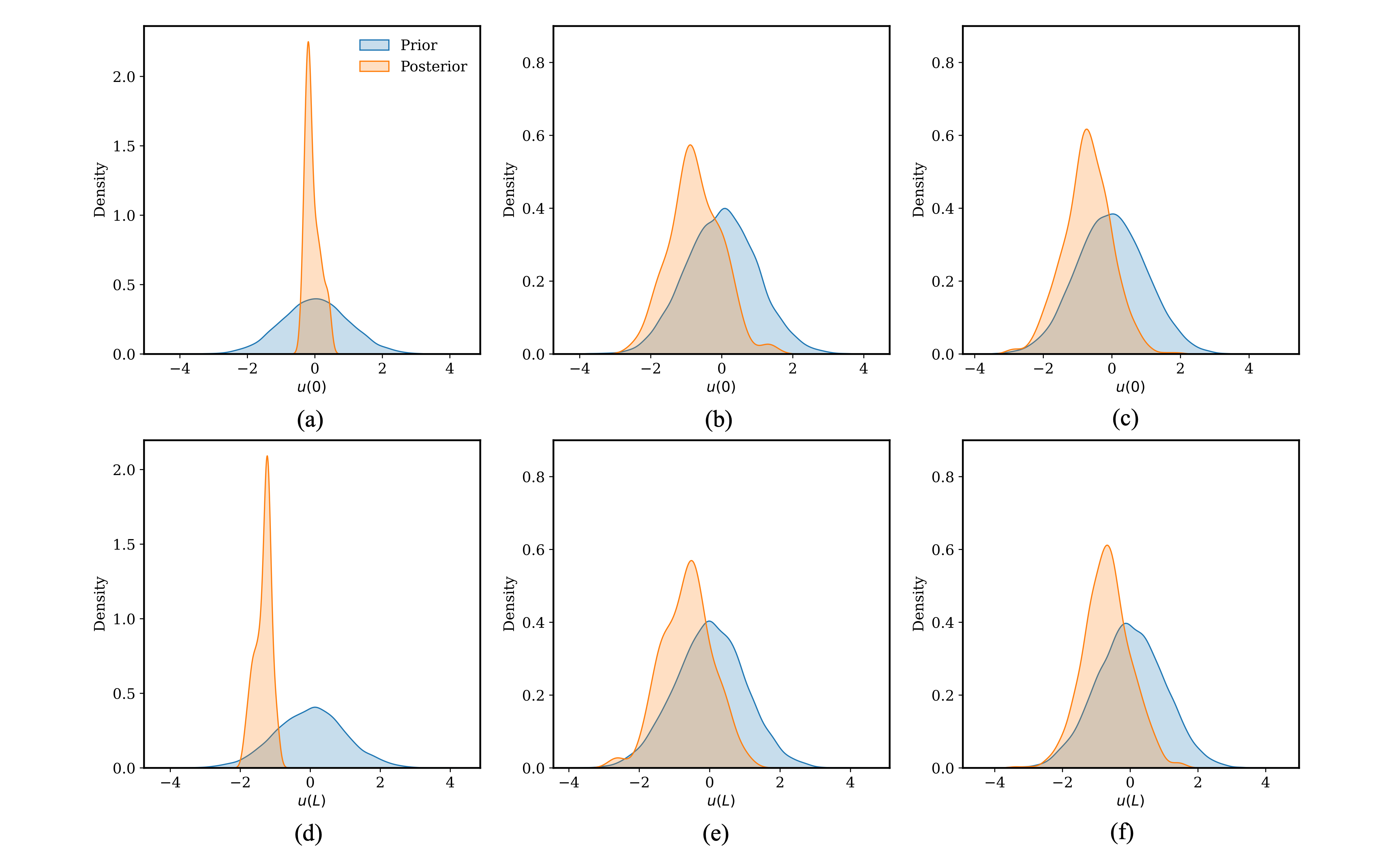
Figure 3: Posterior distributions for the diffusion time derivative problem when inferring only the model parameters. (a), (b) and (c) are the $u_{\mathrm{left}}$ posteriors using IMH, SS, and DES samplers, respectively. (d), (e) and (f) are the $u_{\mathrm{right}}$ posteriors using IMH, SS, and DES samplers, respectively.

When inferring both boundary conditions and the $\sigma$ term, only the SS and DES samplers are considered given the poor performance of the IMH sampler evidenced from the above case. Again, 1,000 serial steps are simulated with 5 parallel proposals per step. Sampling diagnostics are presented for the two samplers in Table 2. The $\tau_p$ for both samplers are comparable, and the $\tau_p$ for DES increased compared to the previous case of inferring only model parameters, possible caused by the increased problem complexity due to the inclusion of the $\sigma$ term. For the ESS, the DES shows a three time enhancement compared to SS, due to the higher residual sample autocorrelation upon chain thinning.

Table 2: Integrated autocorrelation time ( $\tau_p$ ) and effective sample size (ESS) when inferring both model parameters and the $\sigma$ term.

Algorithm	$\tau_p$	ESS
SS	36.228	51.991
DES	45.542	155.0

Scatter plot of the inferred model parameters $u_{\mathrm{left}}$ and $u_{\mathrm{right}}$ is presented in Figure 4. Again, the two model parameters exhibit almost a perfect correlation which is consistent with the observation in the previous case, due to the ill-posedness of the problem.

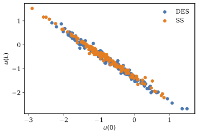
Figure 4: Scatter plot of the samples from IMH, SS, and DES samplers when inferring both model parameters and the $\sigma$ term.

Detailed posterior distributions of $u_{\mathrm{left}}$ , $u_{\mathrm{right}}$ and the $\sigma$ term are presented in Figure 5 for the SS and DES samplers. Both samplers are producing quite consistent posterior distributions. Specifically, Figure 5a and Figure 5d need to be compared for $u_{\mathrm{left}}$ , Figure 5b and Figure 5e for $u_{\mathrm{right}}$ , and Figure 5c and Figure 5f for the $\sigma$ term. Both samplers produce consistent posterior distributions, and the posterior distributions of the $\sigma$ term are approximately centered around the true value of the Gaussian noise (denoted by the solid vertical line) that was added to replicate the “experimental” data.

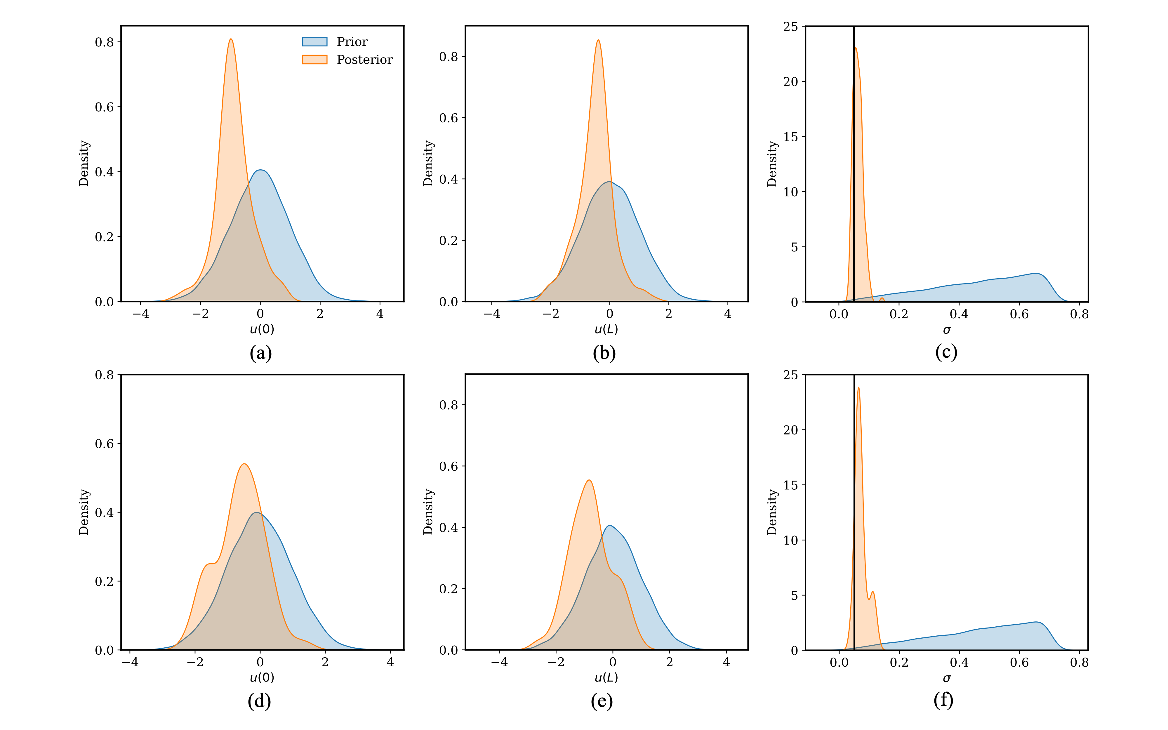
Figure 5: Posterior distributions for the diffusion time derivative problem when inferring the model parameters and the $\sigma$ term. (a), (b) and (c) show the posteriors using SS. (d), (e) and (f) show the posteriors using DES.

As shown in Figure 3 and Figure 5, posteriors of the model parameters and potentially the $\sigma$ term are much more constrained compared to the priors, reflecting the integration of experimental information into the models through the Bayesian UQ process. Followup forward UQ based on the updated posteriors will provide more accurate information about the output uncertainty.

References

C. J. T. Braak. A markov chain monte carlo version of the genetic algorithm differential evolution: easy bayesian computing for real parameter spaces. Statistics and Computing, 16:239–249, 2006. doi:10.1007/s11222-006-8769-1.

@article{braak2006markov,
    author = "Braak, C. J. T.",
    title = "A Markov Chain Monte Carlo version of the genetic algorithm Differential Evolution: easy Bayesian computing for real parameter spaces",
    journal = "Statistics and Computing",
    volume = "16",
    pages = "239--249",
    year = "2006",
    doi = "10.1007/s11222-006-8769-1"
}

B. Calderhead. A general construction for parallelizing metropolis-hastings algorithms. Proceedings of the National Academy of Sciences, 111(49):17408–17413, 2014. doi:10.1073/pnas.1408184111.

@article{calderhead2014general,
    author = "Calderhead, B.",
    title = "A general construction for parallelizing Metropolis-Hastings algorithms",
    journal = "Proceedings of the National Academy of Sciences",
    volume = "111",
    number = "49",
    pages = "17408--17413",
    year = "2014",
    doi = "10.1073/pnas.1408184111"
}

Som LakshmiNarasimha Dhulipala, Daniel Schwen, Yifeng Che, Ryan Terrence Sweet, Aysenur Toptan, Zachary M Prince, Peter German, and Stephen R Novascone. Massively parallel bayesian model calibration and uncertainty quantification with applications to nuclear fuels and materials. Technical Report, Idaho National Laboratory (INL), Idaho Falls, ID (United States), 2023.

@techreport{dhulipala2023massively,
    author = "Dhulipala, Som LakshmiNarasimha and Schwen, Daniel and Che, Yifeng and Sweet, Ryan Terrence and Toptan, Aysenur and Prince, Zachary M and German, Peter and Novascone, Stephen R",
    title = "Massively Parallel Bayesian Model Calibration and Uncertainty Quantification with Applications to Nuclear Fuels and Materials",
    year = "2023",
    institution = "Idaho National Laboratory (INL), Idaho Falls, ID (United States)"
}

J. Goodman and J. Weare. Ensemble samplers with affine invariance. Communications in applied mathematics and computational science, 5(1):65–80, 2010. doi:10.2140/camcos.2010.5.65.

@article{goodman2010ensemble,
    author = "Goodman, J. and Weare, J.",
    title = "Ensemble samplers with affine invariance",
    journal = "Communications in applied mathematics and computational science",
    volume = "5",
    number = "1",
    pages = "65--80",
    year = "2010",
    doi = "10.2140/camcos.2010.5.65"
}

B. Nelson, E. B. Ford, and M. J. Payne. Run dmc: an efficient, parallel code for analyzing radial velocity observations using n-body integrations and differential evolution markov chain monte carlo. The Astrophysical Journal Supplement Series, 11:11–25, 2013. doi:10.1088/0067-0049/210/1/11.

@article{nelson2013rundmc,
    author = "Nelson, B. and Ford, E. B. and Payne, M. J.",
    title = "Run DMC: an efficient, parallel code for analyzing radial velocity observations using n-body integrations and differential evolution Markov chain Monte Carlo",
    journal = "The Astrophysical Journal Supplement Series",
    volume = "11",
    pages = "11--25",
    year = "2013",
    doi = "10.1088/0067-0049/210/1/11"
}

M. D. Shields, D. G. Giovanis, and V. S. Sundar. Subset simulation for problems with strongly non-gaussian, highly anisotropic, and degenerate distributions. Computers & Structures, 245:106431, 2021. doi:10.1016/j.compstruc.2020.106431.

@article{shields2021subset,
    author = "Shields, M. D. and Giovanis, D. G. and Sundar, V. S.",
    title = "Subset simulation for problems with strongly non-Gaussian, highly anisotropic, and degenerate distributions",
    journal = "Computers \\& Structures",
    volume = "245",
    pages = "106431",
    year = "2021",
    doi = "10.1016/j.compstruc.2020.106431"
}

(contrib/moose/modules/stochastic_tools/test/tests/samplers/mcmc/sub.i)

left_bc = 0.13508909593042528
right_bc = -1.5530467809139854
mesh1 = 1

param1 = '${fparse left_bc}'
param2 = '${fparse right_bc}'
param3 = '${fparse mesh1}'

[Mesh]
  type = GeneratedMesh
  dim = 2
  xmax = ${param3}
  xmin = 0
  ymax = 1
  ymin = 0
  nx = 10
  ny = 10
[]

[Variables]
  [u]
  []
[]

[Kernels]
  [diff]
    type = Diffusion
    variable = u
  []
  [time]
    type = TimeDerivative
    variable = u
  []
[]

[BCs]
  [left]
    type = DirichletBC
    variable = u
    boundary = left
    value = ${param1} # Actual = 0.15
  []
  [right]
    type = DirichletBC
    variable = u
    boundary = right
    value = ${param2} # Actual = -1.5
  []
[]

[Postprocessors]
  [average]
    type = ElementAverageValue
    variable = u
  []
[]

[Executioner]
  type = Transient
  num_steps = 5
  dt = 0.1
  solve_type = PJFNK
  petsc_options_iname = '-pc_type -pc_hypre_type'
  petsc_options_value = 'hypre boomeramg'
[]

[Outputs]
  console = 'false'
[]

(contrib/moose/modules/stochastic_tools/test/tests/samplers/mcmc/main_des.i)

[StochasticTools]
[]

[Distributions]
  [left]
    type = Normal
    mean = 0.0
    standard_deviation = 1.0
  []
  [right]
    type = Normal
    mean = 0.0
    standard_deviation = 1.0
  []
[]

[Likelihood]
  [gaussian]
    type = Gaussian
    noise = 'noise_specified/noise_specified'
    file_name = 'exp_0_05.csv'
    log_likelihood = true
  []
[]

[Samplers]
  [sample]
    type = AffineInvariantDES
    prior_distributions = 'left right'
    num_parallel_proposals = 5
    file_name = 'confg.csv'
    execute_on = PRE_MULTIAPP_SETUP
    seed = 2547
    initial_values = '0.1 0.1'
    previous_state = 'mcmc_reporter/inputs'
    previous_state_var = 'mcmc_reporter/variance'
  []
[]

[MultiApps]
  [sub]
    type = SamplerFullSolveMultiApp
    input_files = sub.i
    sampler = sample
  []
[]

[Transfers]
  [reporter_transfer]
    type = SamplerReporterTransfer
    from_reporter = 'average/value'
    stochastic_reporter = 'constant'
    from_multi_app = sub
    sampler = sample
  []
[]

[Controls]
  [cmdline]
    type = MultiAppSamplerControl
    multi_app = sub
    sampler = sample
    param_names = 'left_bc right_bc mesh1'
  []
[]

[Reporters]
  [constant]
    type = StochasticReporter
  []
  [noise_specified]
    type = ConstantReporter
    real_names = 'noise_specified'
    real_values = '0.05'
  []
  [mcmc_reporter]
    type = AffineInvariantDifferentialDecision
    output_value = constant/reporter_transfer:average:value
    sampler = sample
    likelihoods = 'gaussian'
  []
[]

[Executioner]
  type = Transient
  num_steps = 5
[]

[Outputs]
  file_base = 'des_5prop'
  [out]
    type = JSON
    execute_system_information_on = NONE
  []
[]

(contrib/moose/modules/stochastic_tools/test/tests/samplers/mcmc/main_des.i)

[StochasticTools]
[]

[Distributions]
  [left]
    type = Normal
    mean = 0.0
    standard_deviation = 1.0
  []
  [right]
    type = Normal
    mean = 0.0
    standard_deviation = 1.0
  []
[]

[Likelihood]
  [gaussian]
    type = Gaussian
    noise = 'noise_specified/noise_specified'
    file_name = 'exp_0_05.csv'
    log_likelihood = true
  []
[]

[Samplers]
  [sample]
    type = AffineInvariantDES
    prior_distributions = 'left right'
    num_parallel_proposals = 5
    file_name = 'confg.csv'
    execute_on = PRE_MULTIAPP_SETUP
    seed = 2547
    initial_values = '0.1 0.1'
    previous_state = 'mcmc_reporter/inputs'
    previous_state_var = 'mcmc_reporter/variance'
  []
[]

[MultiApps]
  [sub]
    type = SamplerFullSolveMultiApp
    input_files = sub.i
    sampler = sample
  []
[]

[Transfers]
  [reporter_transfer]
    type = SamplerReporterTransfer
    from_reporter = 'average/value'
    stochastic_reporter = 'constant'
    from_multi_app = sub
    sampler = sample
  []
[]

[Controls]
  [cmdline]
    type = MultiAppSamplerControl
    multi_app = sub
    sampler = sample
    param_names = 'left_bc right_bc mesh1'
  []
[]

[Reporters]
  [constant]
    type = StochasticReporter
  []
  [noise_specified]
    type = ConstantReporter
    real_names = 'noise_specified'
    real_values = '0.05'
  []
  [mcmc_reporter]
    type = AffineInvariantDifferentialDecision
    output_value = constant/reporter_transfer:average:value
    sampler = sample
    likelihoods = 'gaussian'
  []
[]

[Executioner]
  type = Transient
  num_steps = 5
[]

[Outputs]
  file_base = 'des_5prop'
  [out]
    type = JSON
    execute_system_information_on = NONE
  []
[]

(contrib/moose/modules/stochastic_tools/test/tests/samplers/mcmc/main_des.i)

[StochasticTools]
[]

[Distributions]
  [left]
    type = Normal
    mean = 0.0
    standard_deviation = 1.0
  []
  [right]
    type = Normal
    mean = 0.0
    standard_deviation = 1.0
  []
[]

[Likelihood]
  [gaussian]
    type = Gaussian
    noise = 'noise_specified/noise_specified'
    file_name = 'exp_0_05.csv'
    log_likelihood = true
  []
[]

[Samplers]
  [sample]
    type = AffineInvariantDES
    prior_distributions = 'left right'
    num_parallel_proposals = 5
    file_name = 'confg.csv'
    execute_on = PRE_MULTIAPP_SETUP
    seed = 2547
    initial_values = '0.1 0.1'
    previous_state = 'mcmc_reporter/inputs'
    previous_state_var = 'mcmc_reporter/variance'
  []
[]

[MultiApps]
  [sub]
    type = SamplerFullSolveMultiApp
    input_files = sub.i
    sampler = sample
  []
[]

[Transfers]
  [reporter_transfer]
    type = SamplerReporterTransfer
    from_reporter = 'average/value'
    stochastic_reporter = 'constant'
    from_multi_app = sub
    sampler = sample
  []
[]

[Controls]
  [cmdline]
    type = MultiAppSamplerControl
    multi_app = sub
    sampler = sample
    param_names = 'left_bc right_bc mesh1'
  []
[]

[Reporters]
  [constant]
    type = StochasticReporter
  []
  [noise_specified]
    type = ConstantReporter
    real_names = 'noise_specified'
    real_values = '0.05'
  []
  [mcmc_reporter]
    type = AffineInvariantDifferentialDecision
    output_value = constant/reporter_transfer:average:value
    sampler = sample
    likelihoods = 'gaussian'
  []
[]

[Executioner]
  type = Transient
  num_steps = 5
[]

[Outputs]
  file_base = 'des_5prop'
  [out]
    type = JSON
    execute_system_information_on = NONE
  []
[]

(contrib/moose/modules/stochastic_tools/test/tests/samplers/mcmc/main_des.i)

[StochasticTools]
[]

[Distributions]
  [left]
    type = Normal
    mean = 0.0
    standard_deviation = 1.0
  []
  [right]
    type = Normal
    mean = 0.0
    standard_deviation = 1.0
  []
[]

[Likelihood]
  [gaussian]
    type = Gaussian
    noise = 'noise_specified/noise_specified'
    file_name = 'exp_0_05.csv'
    log_likelihood = true
  []
[]

[Samplers]
  [sample]
    type = AffineInvariantDES
    prior_distributions = 'left right'
    num_parallel_proposals = 5
    file_name = 'confg.csv'
    execute_on = PRE_MULTIAPP_SETUP
    seed = 2547
    initial_values = '0.1 0.1'
    previous_state = 'mcmc_reporter/inputs'
    previous_state_var = 'mcmc_reporter/variance'
  []
[]

[MultiApps]
  [sub]
    type = SamplerFullSolveMultiApp
    input_files = sub.i
    sampler = sample
  []
[]

[Transfers]
  [reporter_transfer]
    type = SamplerReporterTransfer
    from_reporter = 'average/value'
    stochastic_reporter = 'constant'
    from_multi_app = sub
    sampler = sample
  []
[]

[Controls]
  [cmdline]
    type = MultiAppSamplerControl
    multi_app = sub
    sampler = sample
    param_names = 'left_bc right_bc mesh1'
  []
[]

[Reporters]
  [constant]
    type = StochasticReporter
  []
  [noise_specified]
    type = ConstantReporter
    real_names = 'noise_specified'
    real_values = '0.05'
  []
  [mcmc_reporter]
    type = AffineInvariantDifferentialDecision
    output_value = constant/reporter_transfer:average:value
    sampler = sample
    likelihoods = 'gaussian'
  []
[]

[Executioner]
  type = Transient
  num_steps = 5
[]

[Outputs]
  file_base = 'des_5prop'
  [out]
    type = JSON
    execute_system_information_on = NONE
  []
[]

(contrib/moose/modules/stochastic_tools/test/tests/samplers/mcmc/main_des.i)

[StochasticTools]
[]

[Distributions]
  [left]
    type = Normal
    mean = 0.0
    standard_deviation = 1.0
  []
  [right]
    type = Normal
    mean = 0.0
    standard_deviation = 1.0
  []
[]

[Likelihood]
  [gaussian]
    type = Gaussian
    noise = 'noise_specified/noise_specified'
    file_name = 'exp_0_05.csv'
    log_likelihood = true
  []
[]

[Samplers]
  [sample]
    type = AffineInvariantDES
    prior_distributions = 'left right'
    num_parallel_proposals = 5
    file_name = 'confg.csv'
    execute_on = PRE_MULTIAPP_SETUP
    seed = 2547
    initial_values = '0.1 0.1'
    previous_state = 'mcmc_reporter/inputs'
    previous_state_var = 'mcmc_reporter/variance'
  []
[]

[MultiApps]
  [sub]
    type = SamplerFullSolveMultiApp
    input_files = sub.i
    sampler = sample
  []
[]

[Transfers]
  [reporter_transfer]
    type = SamplerReporterTransfer
    from_reporter = 'average/value'
    stochastic_reporter = 'constant'
    from_multi_app = sub
    sampler = sample
  []
[]

[Controls]
  [cmdline]
    type = MultiAppSamplerControl
    multi_app = sub
    sampler = sample
    param_names = 'left_bc right_bc mesh1'
  []
[]

[Reporters]
  [constant]
    type = StochasticReporter
  []
  [noise_specified]
    type = ConstantReporter
    real_names = 'noise_specified'
    real_values = '0.05'
  []
  [mcmc_reporter]
    type = AffineInvariantDifferentialDecision
    output_value = constant/reporter_transfer:average:value
    sampler = sample
    likelihoods = 'gaussian'
  []
[]

[Executioner]
  type = Transient
  num_steps = 5
[]

[Outputs]
  file_base = 'des_5prop'
  [out]
    type = JSON
    execute_system_information_on = NONE
  []
[]

(contrib/moose/modules/stochastic_tools/test/tests/samplers/mcmc/main_des.i)

[StochasticTools]
[]

[Distributions]
  [left]
    type = Normal
    mean = 0.0
    standard_deviation = 1.0
  []
  [right]
    type = Normal
    mean = 0.0
    standard_deviation = 1.0
  []
[]

[Likelihood]
  [gaussian]
    type = Gaussian
    noise = 'noise_specified/noise_specified'
    file_name = 'exp_0_05.csv'
    log_likelihood = true
  []
[]

[Samplers]
  [sample]
    type = AffineInvariantDES
    prior_distributions = 'left right'
    num_parallel_proposals = 5
    file_name = 'confg.csv'
    execute_on = PRE_MULTIAPP_SETUP
    seed = 2547
    initial_values = '0.1 0.1'
    previous_state = 'mcmc_reporter/inputs'
    previous_state_var = 'mcmc_reporter/variance'
  []
[]

[MultiApps]
  [sub]
    type = SamplerFullSolveMultiApp
    input_files = sub.i
    sampler = sample
  []
[]

[Transfers]
  [reporter_transfer]
    type = SamplerReporterTransfer
    from_reporter = 'average/value'
    stochastic_reporter = 'constant'
    from_multi_app = sub
    sampler = sample
  []
[]

[Controls]
  [cmdline]
    type = MultiAppSamplerControl
    multi_app = sub
    sampler = sample
    param_names = 'left_bc right_bc mesh1'
  []
[]

[Reporters]
  [constant]
    type = StochasticReporter
  []
  [noise_specified]
    type = ConstantReporter
    real_names = 'noise_specified'
    real_values = '0.05'
  []
  [mcmc_reporter]
    type = AffineInvariantDifferentialDecision
    output_value = constant/reporter_transfer:average:value
    sampler = sample
    likelihoods = 'gaussian'
  []
[]

[Executioner]
  type = Transient
  num_steps = 5
[]

[Outputs]
  file_base = 'des_5prop'
  [out]
    type = JSON
    execute_system_information_on = NONE
  []
[]

(contrib/moose/modules/stochastic_tools/test/tests/samplers/mcmc/main_des.i)

[StochasticTools]
[]

[Distributions]
  [left]
    type = Normal
    mean = 0.0
    standard_deviation = 1.0
  []
  [right]
    type = Normal
    mean = 0.0
    standard_deviation = 1.0
  []
[]

[Likelihood]
  [gaussian]
    type = Gaussian
    noise = 'noise_specified/noise_specified'
    file_name = 'exp_0_05.csv'
    log_likelihood = true
  []
[]

[Samplers]
  [sample]
    type = AffineInvariantDES
    prior_distributions = 'left right'
    num_parallel_proposals = 5
    file_name = 'confg.csv'
    execute_on = PRE_MULTIAPP_SETUP
    seed = 2547
    initial_values = '0.1 0.1'
    previous_state = 'mcmc_reporter/inputs'
    previous_state_var = 'mcmc_reporter/variance'
  []
[]

[MultiApps]
  [sub]
    type = SamplerFullSolveMultiApp
    input_files = sub.i
    sampler = sample
  []
[]

[Transfers]
  [reporter_transfer]
    type = SamplerReporterTransfer
    from_reporter = 'average/value'
    stochastic_reporter = 'constant'
    from_multi_app = sub
    sampler = sample
  []
[]

[Controls]
  [cmdline]
    type = MultiAppSamplerControl
    multi_app = sub
    sampler = sample
    param_names = 'left_bc right_bc mesh1'
  []
[]

[Reporters]
  [constant]
    type = StochasticReporter
  []
  [noise_specified]
    type = ConstantReporter
    real_names = 'noise_specified'
    real_values = '0.05'
  []
  [mcmc_reporter]
    type = AffineInvariantDifferentialDecision
    output_value = constant/reporter_transfer:average:value
    sampler = sample
    likelihoods = 'gaussian'
  []
[]

[Executioner]
  type = Transient
  num_steps = 5
[]

[Outputs]
  file_base = 'des_5prop'
  [out]
    type = JSON
    execute_system_information_on = NONE
  []
[]

(contrib/moose/modules/stochastic_tools/test/tests/samplers/mcmc/main_des.i)

[StochasticTools]
[]

[Distributions]
  [left]
    type = Normal
    mean = 0.0
    standard_deviation = 1.0
  []
  [right]
    type = Normal
    mean = 0.0
    standard_deviation = 1.0
  []
[]

[Likelihood]
  [gaussian]
    type = Gaussian
    noise = 'noise_specified/noise_specified'
    file_name = 'exp_0_05.csv'
    log_likelihood = true
  []
[]

[Samplers]
  [sample]
    type = AffineInvariantDES
    prior_distributions = 'left right'
    num_parallel_proposals = 5
    file_name = 'confg.csv'
    execute_on = PRE_MULTIAPP_SETUP
    seed = 2547
    initial_values = '0.1 0.1'
    previous_state = 'mcmc_reporter/inputs'
    previous_state_var = 'mcmc_reporter/variance'
  []
[]

[MultiApps]
  [sub]
    type = SamplerFullSolveMultiApp
    input_files = sub.i
    sampler = sample
  []
[]

[Transfers]
  [reporter_transfer]
    type = SamplerReporterTransfer
    from_reporter = 'average/value'
    stochastic_reporter = 'constant'
    from_multi_app = sub
    sampler = sample
  []
[]

[Controls]
  [cmdline]
    type = MultiAppSamplerControl
    multi_app = sub
    sampler = sample
    param_names = 'left_bc right_bc mesh1'
  []
[]

[Reporters]
  [constant]
    type = StochasticReporter
  []
  [noise_specified]
    type = ConstantReporter
    real_names = 'noise_specified'
    real_values = '0.05'
  []
  [mcmc_reporter]
    type = AffineInvariantDifferentialDecision
    output_value = constant/reporter_transfer:average:value
    sampler = sample
    likelihoods = 'gaussian'
  []
[]

[Executioner]
  type = Transient
  num_steps = 5
[]

[Outputs]
  file_base = 'des_5prop'
  [out]
    type = JSON
    execute_system_information_on = NONE
  []
[]

(contrib/moose/modules/stochastic_tools/test/tests/samplers/mcmc/main_imh.i)

[StochasticTools]
[]

[Distributions]
  [left]
    type = Normal
    mean = 0.0
    standard_deviation = 1.0
  []
  [right]
    type = Normal
    mean = 0.0
    standard_deviation = 1.0
  []
[]

[Likelihood]
  [gaussian]
    type = Gaussian
    noise = 'noise_specified/noise_specified'
    file_name = 'exp_0_05.csv'
    log_likelihood = true
  []
[]

[Samplers]
  [sample]
    type = IndependentGaussianMH
    prior_distributions = 'left right'
    # previous_state = 'mcmc_reporter/inputs'
    num_parallel_proposals = 5
    file_name = 'confg.csv'
    execute_on = PRE_MULTIAPP_SETUP
    seed = 2547
    std_prop = '0.05 0.05'
    initial_values = '0.1 0.1'
    seed_inputs = 'mcmc_reporter/seed_input'
  []
[]

[MultiApps]
  [sub]
    type = SamplerFullSolveMultiApp
    input_files = sub.i
    sampler = sample
  []
[]

[Transfers]
  [reporter_transfer]
    type = SamplerReporterTransfer
    from_reporter = 'average/value'
    stochastic_reporter = 'constant'
    from_multi_app = sub
    sampler = sample
  []
[]

[Controls]
  [cmdline]
    type = MultiAppSamplerControl
    multi_app = sub
    sampler = sample
    param_names = 'left_bc right_bc mesh1'
  []
[]

[Reporters]
  [constant]
    type = StochasticReporter
  []
  [noise_specified]
    type = ConstantReporter
    real_names = 'noise_specified'
    real_values = '0.05'
  []
  [mcmc_reporter]
    type = IndependentMHDecision
    output_value = constant/reporter_transfer:average:value
    sampler = sample
    likelihoods = 'gaussian'
  []
[]

[Executioner]
  type = Transient
  num_steps = 5
[]

[Outputs]
  file_base = 'imh_5prop'
  [out]
    type = JSON
    execute_system_information_on = NONE
  []
[]

(contrib/moose/modules/stochastic_tools/test/tests/samplers/mcmc/main_imh.i)

[StochasticTools]
[]

[Distributions]
  [left]
    type = Normal
    mean = 0.0
    standard_deviation = 1.0
  []
  [right]
    type = Normal
    mean = 0.0
    standard_deviation = 1.0
  []
[]

[Likelihood]
  [gaussian]
    type = Gaussian
    noise = 'noise_specified/noise_specified'
    file_name = 'exp_0_05.csv'
    log_likelihood = true
  []
[]

[Samplers]
  [sample]
    type = IndependentGaussianMH
    prior_distributions = 'left right'
    # previous_state = 'mcmc_reporter/inputs'
    num_parallel_proposals = 5
    file_name = 'confg.csv'
    execute_on = PRE_MULTIAPP_SETUP
    seed = 2547
    std_prop = '0.05 0.05'
    initial_values = '0.1 0.1'
    seed_inputs = 'mcmc_reporter/seed_input'
  []
[]

[MultiApps]
  [sub]
    type = SamplerFullSolveMultiApp
    input_files = sub.i
    sampler = sample
  []
[]

[Transfers]
  [reporter_transfer]
    type = SamplerReporterTransfer
    from_reporter = 'average/value'
    stochastic_reporter = 'constant'
    from_multi_app = sub
    sampler = sample
  []
[]

[Controls]
  [cmdline]
    type = MultiAppSamplerControl
    multi_app = sub
    sampler = sample
    param_names = 'left_bc right_bc mesh1'
  []
[]

[Reporters]
  [constant]
    type = StochasticReporter
  []
  [noise_specified]
    type = ConstantReporter
    real_names = 'noise_specified'
    real_values = '0.05'
  []
  [mcmc_reporter]
    type = IndependentMHDecision
    output_value = constant/reporter_transfer:average:value
    sampler = sample
    likelihoods = 'gaussian'
  []
[]

[Executioner]
  type = Transient
  num_steps = 5
[]

[Outputs]
  file_base = 'imh_5prop'
  [out]
    type = JSON
    execute_system_information_on = NONE
  []
[]

(contrib/moose/modules/stochastic_tools/test/tests/samplers/mcmc/main_ss.i)

[StochasticTools]
[]

[Distributions]
  [left]
    type = Normal
    mean = 0.0
    standard_deviation = 1.0
  []
  [right]
    type = Normal
    mean = 0.0
    standard_deviation = 1.0
  []
[]

[Likelihood]
  [gaussian]
    type = Gaussian
    noise = 'noise_specified/noise_specified'
    file_name = 'exp_0_05.csv'
    log_likelihood = true
  []
[]

[Samplers]
  [sample]
    type = AffineInvariantStretchSampler
    prior_distributions = 'left right'
    num_parallel_proposals = 5
    file_name = 'confg.csv'
    execute_on = PRE_MULTIAPP_SETUP
    seed = 2547
    initial_values = '0.1 0.1'
    previous_state = 'mcmc_reporter/inputs'
    previous_state_var = 'mcmc_reporter/variance'
  []
[]

[MultiApps]
  [sub]
    type = SamplerFullSolveMultiApp
    input_files = sub.i
    sampler = sample
  []
[]

[Transfers]
  [reporter_transfer]
    type = SamplerReporterTransfer
    from_reporter = 'average/value'
    stochastic_reporter = 'constant'
    from_multi_app = sub
    sampler = sample
  []
[]

[Controls]
  [cmdline]
    type = MultiAppSamplerControl
    multi_app = sub
    sampler = sample
    param_names = 'left_bc right_bc mesh1'
  []
[]

[Reporters]
  [constant]
    type = StochasticReporter
  []
  [noise_specified]
    type = ConstantReporter
    real_names = 'noise_specified'
    real_values = '0.05'
  []
  [mcmc_reporter]
    type = AffineInvariantStretchDecision
    output_value = constant/reporter_transfer:average:value
    sampler = sample
    likelihoods = 'gaussian'
  []
[]

[Executioner]
  type = Transient
  num_steps = 5
[]

[Outputs]
  file_base = 'ss_5prop'
  [out]
    type = JSON
    execute_system_information_on = NONE
  []
[]

(contrib/moose/modules/stochastic_tools/test/tests/samplers/mcmc/main_ss.i)

[StochasticTools]
[]

[Distributions]
  [left]
    type = Normal
    mean = 0.0
    standard_deviation = 1.0
  []
  [right]
    type = Normal
    mean = 0.0
    standard_deviation = 1.0
  []
[]

[Likelihood]
  [gaussian]
    type = Gaussian
    noise = 'noise_specified/noise_specified'
    file_name = 'exp_0_05.csv'
    log_likelihood = true
  []
[]

[Samplers]
  [sample]
    type = AffineInvariantStretchSampler
    prior_distributions = 'left right'
    num_parallel_proposals = 5
    file_name = 'confg.csv'
    execute_on = PRE_MULTIAPP_SETUP
    seed = 2547
    initial_values = '0.1 0.1'
    previous_state = 'mcmc_reporter/inputs'
    previous_state_var = 'mcmc_reporter/variance'
  []
[]

[MultiApps]
  [sub]
    type = SamplerFullSolveMultiApp
    input_files = sub.i
    sampler = sample
  []
[]

[Transfers]
  [reporter_transfer]
    type = SamplerReporterTransfer
    from_reporter = 'average/value'
    stochastic_reporter = 'constant'
    from_multi_app = sub
    sampler = sample
  []
[]

[Controls]
  [cmdline]
    type = MultiAppSamplerControl
    multi_app = sub
    sampler = sample
    param_names = 'left_bc right_bc mesh1'
  []
[]

[Reporters]
  [constant]
    type = StochasticReporter
  []
  [noise_specified]
    type = ConstantReporter
    real_names = 'noise_specified'
    real_values = '0.05'
  []
  [mcmc_reporter]
    type = AffineInvariantStretchDecision
    output_value = constant/reporter_transfer:average:value
    sampler = sample
    likelihoods = 'gaussian'
  []
[]

[Executioner]
  type = Transient
  num_steps = 5
[]

[Outputs]
  file_base = 'ss_5prop'
  [out]
    type = JSON
    execute_system_information_on = NONE
  []
[]

(contrib/moose/modules/stochastic_tools/test/tests/samplers/mcmc/main_des.i)

[StochasticTools]
[]

[Distributions]
  [left]
    type = Normal
    mean = 0.0
    standard_deviation = 1.0
  []
  [right]
    type = Normal
    mean = 0.0
    standard_deviation = 1.0
  []
[]

[Likelihood]
  [gaussian]
    type = Gaussian
    noise = 'noise_specified/noise_specified'
    file_name = 'exp_0_05.csv'
    log_likelihood = true
  []
[]

[Samplers]
  [sample]
    type = AffineInvariantDES
    prior_distributions = 'left right'
    num_parallel_proposals = 5
    file_name = 'confg.csv'
    execute_on = PRE_MULTIAPP_SETUP
    seed = 2547
    initial_values = '0.1 0.1'
    previous_state = 'mcmc_reporter/inputs'
    previous_state_var = 'mcmc_reporter/variance'
  []
[]

[MultiApps]
  [sub]
    type = SamplerFullSolveMultiApp
    input_files = sub.i
    sampler = sample
  []
[]

[Transfers]
  [reporter_transfer]
    type = SamplerReporterTransfer
    from_reporter = 'average/value'
    stochastic_reporter = 'constant'
    from_multi_app = sub
    sampler = sample
  []
[]

[Controls]
  [cmdline]
    type = MultiAppSamplerControl
    multi_app = sub
    sampler = sample
    param_names = 'left_bc right_bc mesh1'
  []
[]

[Reporters]
  [constant]
    type = StochasticReporter
  []
  [noise_specified]
    type = ConstantReporter
    real_names = 'noise_specified'
    real_values = '0.05'
  []
  [mcmc_reporter]
    type = AffineInvariantDifferentialDecision
    output_value = constant/reporter_transfer:average:value
    sampler = sample
    likelihoods = 'gaussian'
  []
[]

[Executioner]
  type = Transient
  num_steps = 5
[]

[Outputs]
  file_base = 'des_5prop'
  [out]
    type = JSON
    execute_system_information_on = NONE
  []
[]

(contrib/moose/modules/stochastic_tools/test/tests/samplers/mcmc/main_des.i)

[StochasticTools]
[]

[Distributions]
  [left]
    type = Normal
    mean = 0.0
    standard_deviation = 1.0
  []
  [right]
    type = Normal
    mean = 0.0
    standard_deviation = 1.0
  []
[]

[Likelihood]
  [gaussian]
    type = Gaussian
    noise = 'noise_specified/noise_specified'
    file_name = 'exp_0_05.csv'
    log_likelihood = true
  []
[]

[Samplers]
  [sample]
    type = AffineInvariantDES
    prior_distributions = 'left right'
    num_parallel_proposals = 5
    file_name = 'confg.csv'
    execute_on = PRE_MULTIAPP_SETUP
    seed = 2547
    initial_values = '0.1 0.1'
    previous_state = 'mcmc_reporter/inputs'
    previous_state_var = 'mcmc_reporter/variance'
  []
[]

[MultiApps]
  [sub]
    type = SamplerFullSolveMultiApp
    input_files = sub.i
    sampler = sample
  []
[]

[Transfers]
  [reporter_transfer]
    type = SamplerReporterTransfer
    from_reporter = 'average/value'
    stochastic_reporter = 'constant'
    from_multi_app = sub
    sampler = sample
  []
[]

[Controls]
  [cmdline]
    type = MultiAppSamplerControl
    multi_app = sub
    sampler = sample
    param_names = 'left_bc right_bc mesh1'
  []
[]

[Reporters]
  [constant]
    type = StochasticReporter
  []
  [noise_specified]
    type = ConstantReporter
    real_names = 'noise_specified'
    real_values = '0.05'
  []
  [mcmc_reporter]
    type = AffineInvariantDifferentialDecision
    output_value = constant/reporter_transfer:average:value
    sampler = sample
    likelihoods = 'gaussian'
  []
[]

[Executioner]
  type = Transient
  num_steps = 5
[]

[Outputs]
  file_base = 'des_5prop'
  [out]
    type = JSON
    execute_system_information_on = NONE
  []
[]

(contrib/moose/modules/stochastic_tools/test/tests/samplers/mcmc/main_des_var.i)

[StochasticTools]
[]

[Distributions]
  [left]
    type = Normal
    mean = 0.0
    standard_deviation = 1.0
  []
  [right]
    type = Normal
    mean = 0.0
    standard_deviation = 1.0
  []
  [variance]
    type = Uniform
    lower_bound = 0.0
    upper_bound = 0.5
  []
[]

[Likelihood]
  [gaussian]
    type = Gaussian
    noise = 'mcmc_reporter/noise'
    file_name = 'exp_0_05.csv'
    log_likelihood = true
  []
[]

[Samplers]
  [sample]
    type = AffineInvariantDES
    prior_distributions = 'left right'
    num_parallel_proposals = 5
    file_name = 'confg.csv'
    execute_on = PRE_MULTIAPP_SETUP
    seed = 2547
    initial_values = '0.1 0.1'
    previous_state = 'mcmc_reporter/inputs'
    previous_state_var = 'mcmc_reporter/variance'
    prior_variance = 'variance'
  []
[]

[MultiApps]
  [sub]
    type = SamplerFullSolveMultiApp
    input_files = sub.i
    sampler = sample
  []
[]

[Transfers]
  [reporter_transfer]
    type = SamplerReporterTransfer
    from_reporter = 'average/value'
    stochastic_reporter = 'constant'
    from_multi_app = sub
    sampler = sample
  []
[]

[Controls]
  [cmdline]
    type = MultiAppSamplerControl
    multi_app = sub
    sampler = sample
    param_names = 'left_bc right_bc mesh1'
  []
[]

[Reporters]
  [constant]
    type = StochasticReporter
  []
  [mcmc_reporter]
    type = AffineInvariantDifferentialDecision
    output_value = constant/reporter_transfer:average:value
    sampler = sample
    likelihoods = 'gaussian'
  []
[]

[Executioner]
  type = Transient
  num_steps = 5
[]

[Outputs]
  file_base = 'des_5prop_var'
  [out]
    type = JSON
    execute_system_information_on = NONE
  []
[]

(contrib/moose/modules/stochastic_tools/test/tests/samplers/mcmc/main_des_var.i)

[StochasticTools]
[]

[Distributions]
  [left]
    type = Normal
    mean = 0.0
    standard_deviation = 1.0
  []
  [right]
    type = Normal
    mean = 0.0
    standard_deviation = 1.0
  []
  [variance]
    type = Uniform
    lower_bound = 0.0
    upper_bound = 0.5
  []
[]

[Likelihood]
  [gaussian]
    type = Gaussian
    noise = 'mcmc_reporter/noise'
    file_name = 'exp_0_05.csv'
    log_likelihood = true
  []
[]

[Samplers]
  [sample]
    type = AffineInvariantDES
    prior_distributions = 'left right'
    num_parallel_proposals = 5
    file_name = 'confg.csv'
    execute_on = PRE_MULTIAPP_SETUP
    seed = 2547
    initial_values = '0.1 0.1'
    previous_state = 'mcmc_reporter/inputs'
    previous_state_var = 'mcmc_reporter/variance'
    prior_variance = 'variance'
  []
[]

[MultiApps]
  [sub]
    type = SamplerFullSolveMultiApp
    input_files = sub.i
    sampler = sample
  []
[]

[Transfers]
  [reporter_transfer]
    type = SamplerReporterTransfer
    from_reporter = 'average/value'
    stochastic_reporter = 'constant'
    from_multi_app = sub
    sampler = sample
  []
[]

[Controls]
  [cmdline]
    type = MultiAppSamplerControl
    multi_app = sub
    sampler = sample
    param_names = 'left_bc right_bc mesh1'
  []
[]

[Reporters]
  [constant]
    type = StochasticReporter
  []
  [mcmc_reporter]
    type = AffineInvariantDifferentialDecision
    output_value = constant/reporter_transfer:average:value
    sampler = sample
    likelihoods = 'gaussian'
  []
[]

[Executioner]
  type = Transient
  num_steps = 5
[]

[Outputs]
  file_base = 'des_5prop_var'
  [out]
    type = JSON
    execute_system_information_on = NONE
  []
[]

(contrib/moose/modules/stochastic_tools/test/tests/samplers/mcmc/main_des_var.i)

[StochasticTools]
[]

[Distributions]
  [left]
    type = Normal
    mean = 0.0
    standard_deviation = 1.0
  []
  [right]
    type = Normal
    mean = 0.0
    standard_deviation = 1.0
  []
  [variance]
    type = Uniform
    lower_bound = 0.0
    upper_bound = 0.5
  []
[]

[Likelihood]
  [gaussian]
    type = Gaussian
    noise = 'mcmc_reporter/noise'
    file_name = 'exp_0_05.csv'
    log_likelihood = true
  []
[]

[Samplers]
  [sample]
    type = AffineInvariantDES
    prior_distributions = 'left right'
    num_parallel_proposals = 5
    file_name = 'confg.csv'
    execute_on = PRE_MULTIAPP_SETUP
    seed = 2547
    initial_values = '0.1 0.1'
    previous_state = 'mcmc_reporter/inputs'
    previous_state_var = 'mcmc_reporter/variance'
    prior_variance = 'variance'
  []
[]

[MultiApps]
  [sub]
    type = SamplerFullSolveMultiApp
    input_files = sub.i
    sampler = sample
  []
[]

[Transfers]
  [reporter_transfer]
    type = SamplerReporterTransfer
    from_reporter = 'average/value'
    stochastic_reporter = 'constant'
    from_multi_app = sub
    sampler = sample
  []
[]

[Controls]
  [cmdline]
    type = MultiAppSamplerControl
    multi_app = sub
    sampler = sample
    param_names = 'left_bc right_bc mesh1'
  []
[]

[Reporters]
  [constant]
    type = StochasticReporter
  []
  [mcmc_reporter]
    type = AffineInvariantDifferentialDecision
    output_value = constant/reporter_transfer:average:value
    sampler = sample
    likelihoods = 'gaussian'
  []
[]

[Executioner]
  type = Transient
  num_steps = 5
[]

[Outputs]
  file_base = 'des_5prop_var'
  [out]
    type = JSON
    execute_system_information_on = NONE
  []
[]

(contrib/moose/modules/stochastic_tools/test/tests/samplers/mcmc/main_des_var.i)

[StochasticTools]
[]

[Distributions]
  [left]
    type = Normal
    mean = 0.0
    standard_deviation = 1.0
  []
  [right]
    type = Normal
    mean = 0.0
    standard_deviation = 1.0
  []
  [variance]
    type = Uniform
    lower_bound = 0.0
    upper_bound = 0.5
  []
[]

[Likelihood]
  [gaussian]
    type = Gaussian
    noise = 'mcmc_reporter/noise'
    file_name = 'exp_0_05.csv'
    log_likelihood = true
  []
[]

[Samplers]
  [sample]
    type = AffineInvariantDES
    prior_distributions = 'left right'
    num_parallel_proposals = 5
    file_name = 'confg.csv'
    execute_on = PRE_MULTIAPP_SETUP
    seed = 2547
    initial_values = '0.1 0.1'
    previous_state = 'mcmc_reporter/inputs'
    previous_state_var = 'mcmc_reporter/variance'
    prior_variance = 'variance'
  []
[]

[MultiApps]
  [sub]
    type = SamplerFullSolveMultiApp
    input_files = sub.i
    sampler = sample
  []
[]

[Transfers]
  [reporter_transfer]
    type = SamplerReporterTransfer
    from_reporter = 'average/value'
    stochastic_reporter = 'constant'
    from_multi_app = sub
    sampler = sample
  []
[]

[Controls]
  [cmdline]
    type = MultiAppSamplerControl
    multi_app = sub
    sampler = sample
    param_names = 'left_bc right_bc mesh1'
  []
[]

[Reporters]
  [constant]
    type = StochasticReporter
  []
  [mcmc_reporter]
    type = AffineInvariantDifferentialDecision
    output_value = constant/reporter_transfer:average:value
    sampler = sample
    likelihoods = 'gaussian'
  []
[]

[Executioner]
  type = Transient
  num_steps = 5
[]

[Outputs]
  file_base = 'des_5prop_var'
  [out]
    type = JSON
    execute_system_information_on = NONE
  []
[]

Overview of Bayesian UQ
Problem Statement
Inferring Calibration Parameters Only ( Fixed Term ) var element = document.getElementById("moose-equation-a2a1dc4a-244a-4910-b127-65c6308ac381");katex.render("\\sigma", element, {displayMode:false,throwOnError:false});
Inferring Both Calibration Parameters and the Variance Term
Result and Analysis
References

Bayesian Uncertainty Quantification (UQ) on a 1D Diffusion Problem

Overview of Bayesian UQ

Problem Statement

Inferring Calibration Parameters Only (Fixed σ\sigmaσ Term)

Sub-Application Input

Main Input

Available Sampling Algorithms

Inferring Both Calibration Parameters and the Variance Term

Result and Analysis

References

(contrib/moose/modules/stochastic_tools/test/tests/samplers/mcmc/sub.i)

(contrib/moose/modules/stochastic_tools/test/tests/samplers/mcmc/main_des.i)

(contrib/moose/modules/stochastic_tools/test/tests/samplers/mcmc/main_des.i)

(contrib/moose/modules/stochastic_tools/test/tests/samplers/mcmc/main_des.i)

(contrib/moose/modules/stochastic_tools/test/tests/samplers/mcmc/main_des.i)

(contrib/moose/modules/stochastic_tools/test/tests/samplers/mcmc/main_des.i)

(contrib/moose/modules/stochastic_tools/test/tests/samplers/mcmc/main_des.i)

(contrib/moose/modules/stochastic_tools/test/tests/samplers/mcmc/main_des.i)

(contrib/moose/modules/stochastic_tools/test/tests/samplers/mcmc/main_des.i)

(contrib/moose/modules/stochastic_tools/test/tests/samplers/mcmc/main_imh.i)

(contrib/moose/modules/stochastic_tools/test/tests/samplers/mcmc/main_imh.i)

(contrib/moose/modules/stochastic_tools/test/tests/samplers/mcmc/main_ss.i)

(contrib/moose/modules/stochastic_tools/test/tests/samplers/mcmc/main_ss.i)

(contrib/moose/modules/stochastic_tools/test/tests/samplers/mcmc/main_des.i)

(contrib/moose/modules/stochastic_tools/test/tests/samplers/mcmc/main_des.i)

(contrib/moose/modules/stochastic_tools/test/tests/samplers/mcmc/main_des_var.i)

(contrib/moose/modules/stochastic_tools/test/tests/samplers/mcmc/main_des_var.i)

(contrib/moose/modules/stochastic_tools/test/tests/samplers/mcmc/main_des_var.i)

(contrib/moose/modules/stochastic_tools/test/tests/samplers/mcmc/main_des_var.i)

Inferring Calibration Parameters Only (Fixed $\sigma$ Term)